Spatial corrections

In order to include the spatial corrections to the mass resolution we recorded the mean of the $V_s(M^2)/M^4$ distributions for each ($E_1,E_2$) bin for both the $\eta$ and $\pi ^0$ samples. Then we modified the expression for the variance function (Eq. (3)), using Eq. (4) for the contribution from energy resolution,

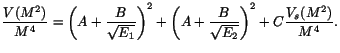$$\frac{V(M^2)}{M^4} = \left(A + \frac{B}{\sqrt{E_1}}\right)^2 + \left(A + \frac{B}{\sqrt{E_2}}\right)^2 + C \frac{V_s(M^2)}{M^4}.$$ (10)

In addition to the standard parameters $A$ and $B$, we introduced parameter $C$ that scales the spatial resolution contribution. With this simple model we first fitted $\eta$ data with $C$ set to zero. The fit is shown as the solid line in Fig. 8, while the fit parameters are shown in the first row of Table 2. Next we let $C$ vary. The corresponding fit is represented by the dashed line in Fig. 8 and the second row in Table 2. The fit confirms that the $\eta$ mass is not very sensitive to spatial corrections. In the next step we fitted all measured points from the $\eta$ and $\pi ^0$ samples together. The fit is shown as the dotted line in Fig. 8, and the resulting parameters are shown in the last row of Table 2. Both the $\pi ^0$ and $\eta$ mass distributions are described well by the model. We used a single parameter to scale the spatial contribution to the mass resolution. The energy-dependent part of the spatial error in Eq. (7) is dominant at small and moderate angles $\theta \approx 10\deg$, while the angular part in Eq. (7) becomes more important at large angles $\theta> 15\deg$. We checked the importance of the angle-dependent spatial errors by setting $X_0 = 0$ in Eq. (7), which made the overall $\chi ^2$ worse. We conclude that it is important to use elliptically errors at larger angles. The scale parameter $C$ can be viewed as a correction to the nominal value of $C_E = 7.1$ mm$\cdot$GeV $^{\frac{1}{2}}$ for the LGD.

Table 2: The parameter values from different fits to the $\eta$ and $\pi ^0$ mass resolutions, obtained using Eq. (10). The corresponding fits are shown in Fig. 8

Fit	$A$	$B$ $\left[GeV^{-1/2}\right]$	$C$	$\chi ^2$
$\eta$ ($C=0$)	$0.0371\pm0.0006$	$0.0797\pm0.0008$	0	1.05
$\eta$ (full)	$0.036\pm0.008$	$0.080\pm0.003$	$0.26\pm1.76$	1.04
$\eta+\pi^0$ (full)	$0.035\pm0.004$	$0.073\pm0.006$	$0.90\pm0.02$	1.50

Figure 3: Energy distribution of $E_1$ vs. $E_2$ (red boxes). Green dots represent showers with invariant mass close to the $\pi ^0$ mass (right) and $\eta$ mass (left). Black dots represent the pairs of photon energies for which $V(M^2)$ has been fitted. Solid lines correspond to the case when $E_1 =E_2$.

Figure 4: The $\eta$ squared-mass distributions for 9 energy bins, fitted with a Gaussian. The dotted lines represent a polynomial background. Below each plot are shown the corresponding energies ($E_1,E_2$).

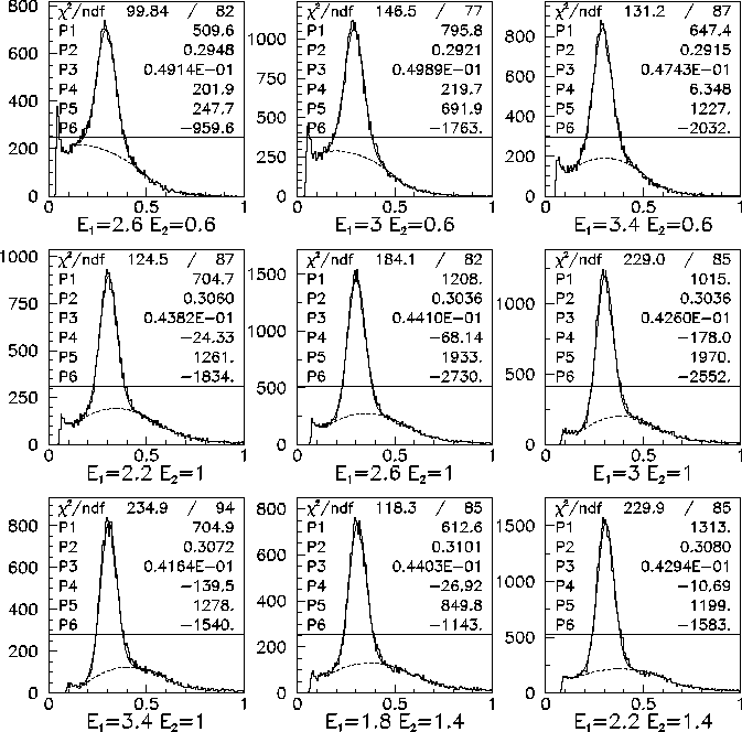Figure 5: The same as Fig. 4 for energy bins $10-18$.

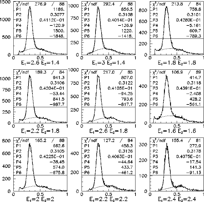Figure 6: The $\pi ^0$ mass distribution for 8 energy bins, fitted with a Gaussian. The dotted lines represent a polynomial background.

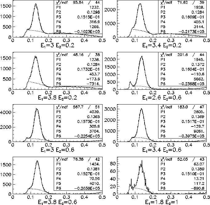Figure 7: The same as Fig. 6 for energy bins $9-16$.

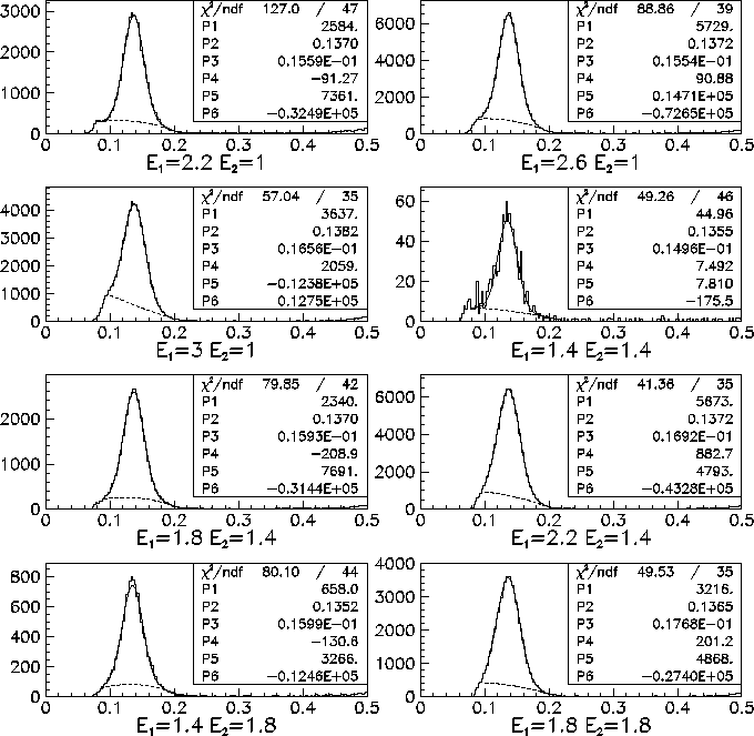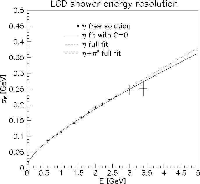
Figure 8: Energy resolution of showers in the LGD obtained from analysis of the $2\gamma$ sample. Points represent the free solution to the $\eta$ squared-mass resolution measurements when the contribution from the spatial resolution has been neglected. The solid line represents the fit to the $\eta$ data with the standard energy resolution model (Eq. (10)with $C=0$). The dashed line represents the fit to the $\eta$ data when the spatial contribution is taken into account by Eq. (10). The dotted line corresponds to the simultaneous fit to the $\eta$ and $\pi ^0$ data with the same function (Eq. (10)). Corresponding fit parameters and $\chi ^2$ are shown in Table 2.