


Next: The energy resolution
Up: report
Previous: Introduction
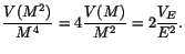
The square of the invariant mass of two photons is given by
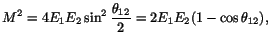 |
(1) |
where  and
and  are corresponding photon energies, while
 is their angular separation. The expression for the variance
of the squared invariant mass in terms of the variances of energy and
shower position in the LGD is given by
is their angular separation. The expression for the variance
of the squared invariant mass in terms of the variances of energy and
shower position in the LGD is given by
![$\displaystyle V(M^2) = \sum_{i=1}^{2} \left[ \
\left(\frac{\partial M^2}{\part...
...rtial x_i}\right)\left(\frac{\partial M^2}{\partial y_i}\right) V_{XY} \right],$](img22.png) |
(2) |
where index  counts photons. Taking all derivatives of Eq. (1)
one can re-write Eq. (2) in the form
counts photons. Taking all derivatives of Eq. (1)
one can re-write Eq. (2) in the form
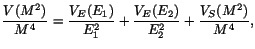 |
(3) |
where spatial derivatives and variances are grouped into the term  .
The usual expression for the energy resolution function is given by [1]
.
The usual expression for the energy resolution function is given by [1]
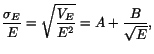 |
(4) |
where parameters  and
and  have to be determined. Spatial derivatives
can be expressed in terms of measured photon momenta utilizing the expression
have to be determined. Spatial derivatives
can be expressed in terms of measured photon momenta utilizing the expression
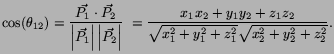 |
(5) |
For example
![$\displaystyle \frac{\partial M^2}{\partial x_1} = -2E_1E_2\frac{\partial \cos(\...
...(P_{y_1}^2 + P_{z_1}^2) \
- P_{x_1}(P_{y_1}P_{y_2} + P_{z_1}P_{z_2} ) \right].$](img30.png) |
(6) |
The other spatial derivatives have a similar form and they can be
obtained by the proper variable substitution. The  position of
the shower maximum is not directly measured. However, it is correlated
with the energy and this has been taken into account within the
shower-depth and nonlinearity corrections [2]. For the
purpose of this analysis a common -plane is fixed at
position of
the shower maximum is not directly measured. However, it is correlated
with the energy and this has been taken into account within the
shower-depth and nonlinearity corrections [2]. For the
purpose of this analysis a common -plane is fixed at 
 .
The fluctuations in the shower position that determine
.
The fluctuations in the shower position that determine  ,
,  and
and
 are also affected by the energy. The energy dependence is
proportional to
are also affected by the energy. The energy dependence is
proportional to
 with a proportionality constant that
depends on the size of the LGD block [3]. This term alone
would make spatial errors cylindrical and uniform across the face of the LGD.
However, one can expect that the uncertainty in the shower position increases
with polar angle
with a proportionality constant that
depends on the size of the LGD block [3]. This term alone
would make spatial errors cylindrical and uniform across the face of the LGD.
However, one can expect that the uncertainty in the shower position increases
with polar angle  , as
, as
 , where
  is the radiation
length of the lead glass. This makes shower centroid errors elliptical.
The orientation of the ellipse depends on the shower azimuthal angle
is the radiation
length of the lead glass. This makes shower centroid errors elliptical.
The orientation of the ellipse depends on the shower azimuthal angle  ,
and is connected with the correlation term . Combining all together,
,
and is connected with the correlation term . Combining all together,
with  mm
mm GeV
GeV
 , and
, and
 mm[4].
In this study, we analyze events with two reconstructed showers. The
mm[4].
In this study, we analyze events with two reconstructed showers. The  sample, consisting of
  events, is selected by limiting invariant mass
to
events, is selected by limiting invariant mass
to 
 . The corresponding invariant mass distribution is shown
on the left side of Fig. 1. The
. The corresponding invariant mass distribution is shown
on the left side of Fig. 1. The  sample is obtained by selecting
pairs with shower separation
sample is obtained by selecting
pairs with shower separation
 . This distance
is approximately twice the average shower size in the LGD plane. The
corresponding mass distribution, shown on the right side of Fig. 1,
contains
. This distance
is approximately twice the average shower size in the LGD plane. The
corresponding mass distribution, shown on the right side of Fig. 1,
contains  events. Small peak around 0.2 represents the
remnants that have large shower separation. The and peaks are
fitted with a Gaussian over a polynomial background. In order to check the
influence of spatial resolution on the overall mass resolution, the distribution
of
events. Small peak around 0.2 represents the
remnants that have large shower separation. The and peaks are
fitted with a Gaussian over a polynomial background. In order to check the
influence of spatial resolution on the overall mass resolution, the distribution
of
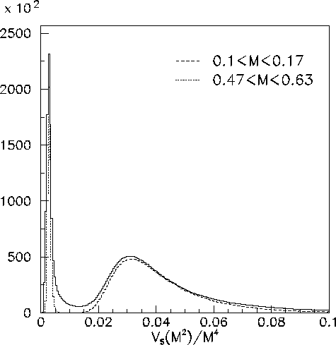
 is plotted in Fig. 2 (solid line), calculated with
the help of Eqs. (6) and (7). The distribution is obtained
from the inclusive
is plotted in Fig. 2 (solid line), calculated with
the help of Eqs. (6) and (7). The distribution is obtained
from the inclusive  sample without restrictions on
  or
or
 . The dotted and dashed lines represent pairs with
invariant mass within a
. The dotted and dashed lines represent pairs with
invariant mass within a  window around the and
peaks, respectively. Table 1 shows the Gaussian mean
and r.m.s. of the two fitted meson peaks from Fig. 1.
The third column represents the
window around the and
peaks, respectively. Table 1 shows the Gaussian mean
and r.m.s. of the two fitted meson peaks from Fig. 1.
The third column represents the
 obtained from the fit. (see
Eq. (8)). The last column represents the mean value of
from the dashed and dotted distributions in Fig 2.
One can see that the spatial resolution contributes about
obtained from the fit. (see
Eq. (8)). The last column represents the mean value of
from the dashed and dotted distributions in Fig 2.
One can see that the spatial resolution contributes about  to the
variance, while the width is affected at the level of
to the
variance, while the width is affected at the level of  .
When two showers have the same energies and the spatial term is small,
Eq. (3) is reduced to
.
When two showers have the same energies and the spatial term is small,
Eq. (3) is reduced to
 |
(8) |
By measuring the mass or squared mass resolution in narrow energy bins one can
extract the energy resolution function Eq. (4) and the corresponding
parameters. The energy bins should be narrower than the detector energy resolution.
Figure 1:
Invariant mass distribution of
 (left) and
 (right).
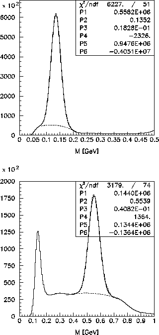 |
Table 1:
The mean,  and corresponding
obtained from the fit
of the two meson peaks in Fig. 1. The last column is the mean
of dashed and dotted distributions from Fig 2, respectively.
and corresponding
obtained from the fit
of the two meson peaks in Fig. 1. The last column is the mean
of dashed and dotted distributions from Fig 2, respectively.
| Data |

![$ \left[GeV\right]$](img66.png) |

|
|
|
|
0.1352 |
0.0183 |
0.0731 |
0.0406 |
|
0.5539 |
0.0408 |
0.0217 |
0.0030 |
Figure 2:
The
 distribution in events calculated using
Eqs. (6) and (7). The dashed and dotted lines represent
the distribution for pairs with mass within the and windows,
respectively.
distribution in events calculated using
Eqs. (6) and (7). The dashed and dotted lines represent
the distribution for pairs with mass within the and windows,
respectively.
 |
Next: The energy resolution
Up: report
Previous: Introduction
Richard T. Jones
2003-10-04