


Next: Spatial corrections
Up: report
Previous: The invariant mass resolution
Fig. 3 shows the energy distribution of the harder shower ( )
vs. the softer shower (
)
vs. the softer shower ( ) for the
  samples. Showers with
separation
samples. Showers with
separation

 are shown on the left, while
pairs with
are shown on the left, while
pairs with 
 are plotted on the right of Fig. 3.
Green dots represent the pairs with masses inside the respective meson
window. Solid lines represent the case where
are plotted on the right of Fig. 3.
Green dots represent the pairs with masses inside the respective meson
window. Solid lines represent the case where  . Fig. 3
shows that the statistics of pairs with is quite poor and
covers a restricted energy range. Consequently, we measured
. Fig. 3
shows that the statistics of pairs with is quite poor and
covers a restricted energy range. Consequently, we measured  for
the set of (
for
the set of ( ) values shown as black dots in Fig. 3.
For each dot, the squared mass distribution (
) values shown as black dots in Fig. 3.
For each dot, the squared mass distribution ( sample) or the invariant
mass distribution (
sample) or the invariant
mass distribution ( data) has been created. Energy limits for a dot
have been chosen to be the
data) has been created. Energy limits for a dot
have been chosen to be the
 for each
  , where
  is deduced from Eq. (4) with
  and
and
 Gev
Gev
 . These
distributions, shown in Figs. 4 - 7, are all fitted
with a Gaussian over a polynomial background. Fitting errors reflect the
statistics of the data sample. Systematic errors are governed by the
choice of background function, and they are estimated to be
. These
distributions, shown in Figs. 4 - 7, are all fitted
with a Gaussian over a polynomial background. Fitting errors reflect the
statistics of the data sample. Systematic errors are governed by the
choice of background function, and they are estimated to be  and
and  for the and data respectively. Reducing the energy bins to
 did not have a significant impact on the results; it only
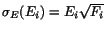
reduced statistics. From the Gaussian fit the value
did not have a significant impact on the results; it only
reduced statistics. From the Gaussian fit the value
 has been
calculated.
In the first approximation, for the data we neglected the spatial
contribution to the mass resolution. Following Eq. (3) we formed
the set of equations
has been
calculated.
In the first approximation, for the data we neglected the spatial
contribution to the mass resolution. Following Eq. (3) we formed
the set of equations
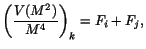 |
(9) |
where
 labels calculated values. We try to solve these
equations for the set of
labels calculated values. We try to solve these
equations for the set of  values, with
 numbering
the selected photon energies. The least-square solution we obtained is
model-independent since we have not presumed the functional form of
numbering
the selected photon energies. The least-square solution we obtained is
model-independent since we have not presumed the functional form of  .
It is free of any restrictions on the
.
It is free of any restrictions on the  values except that
  for
for  . The corresponding
 from the
free solution is plotted in Fig. 8. These points agree very well
with the standard expression for the energy resolution (Eq. 4),
with
from the
free solution is plotted in Fig. 8. These points agree very well
with the standard expression for the energy resolution (Eq. 4),
with  and
and  GeV
.
GeV
.
Next: Spatial corrections
Up: report
Previous: The invariant mass resolution
Richard T. Jones
2003-10-04