


Next: Discussion
Up: psf
Previous: Introduction
There are various functions that have been used to describe the shape of
showers in EM calorimeters. Usually one uses a sum of 2 functions:
a core part that describes the peak of the energy distribution and a
second one that covers the tail. Among others, two exponential, exponential
and Gaussian, and two Gaussian functions have been exploited [2].
The single shower fitter is built to use an arbitrary PSF function without
changing the algorithm.
The first step in fitting an event is to get initial values for the fitting
parameters,
 , from the data. In the case of an isolated shower,
E is set to the total energy in the LGD,
, from the data. In the case of an isolated shower,
E is set to the total energy in the LGD,  , while
  is set by the coordinates of the block with maximum energy yield.
The fit is performed using MINIUT. In order to speed up fitting, we decided not
to fit the whole LGD array, but rather a matrix (currently 9X9) around
the maximum energy block. The fitter minimizes
is set by the coordinates of the block with maximum energy yield.
The fit is performed using MINIUT. In order to speed up fitting, we decided not
to fit the whole LGD array, but rather a matrix (currently 9X9) around
the maximum energy block. The fitter minimizes 
 |
(1) |
where  is the observed block energy, and
  is the PSF function taken
at the center of the block. Errors
is the PSF function taken
at the center of the block. Errors  in Eq. 1 are calculated
from expression
in Eq. 1 are calculated
from expression
 |
(2) |
with A=0.08 and B=0.01.
The first trial function to be used is a single Gaussian
 |
(3) |
with  being the radial distance from the shower center
 .
The normalization
.
The normalization  is determined by the the shower energy E,
N = E/(2
is determined by the the shower energy E,
N = E/(2  ). In order to get the proper overall normalization
one has to multiply Eq. 3 with the LGD block area
). In order to get the proper overall normalization
one has to multiply Eq. 3 with the LGD block area  .
The radial Gaussian width
.
The radial Gaussian width  should be fixed, but can be a function
of energy E and angle
should be fixed, but can be a function
of energy E and angle  . In Fig. 1 is shown how R converges,
when it is used as a free parameter, to the value
. In Fig. 1 is shown how R converges,
when it is used as a free parameter, to the value
 while
shower energy increases. For
while
shower energy increases. For  GeV, is almost independent
of energy. It seems this is a feature of MC showers, connected with the fact
that core contribution, consisting of just two central blocks,
is much more prominent than the tail. We will try to explain this later.
An additional result from the first fit is that the fitted energy is biased
by
GeV, is almost independent
of energy. It seems this is a feature of MC showers, connected with the fact
that core contribution, consisting of just two central blocks,
is much more prominent than the tail. We will try to explain this later.
An additional result from the first fit is that the fitted energy is biased
by
 towards lower values with respect to the generated energy.
Figure 1:
Radial width vs. energy for 0.1, 0.5, 1.0, 2.0, 3.0, 3.5  photons shot in the direction of
 . Left:
initial
. Left:
initial  ,
,  . Right: initial
  ,
,  .
Note: when is allow to vary,
.
Note: when is allow to vary,  has to be large in order to
stabilize fitter and get physically acceptable fits.
has to be large in order to
stabilize fitter and get physically acceptable fits.
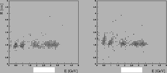 |
Figure 2:
Fit-data difference, averaged over 100 shots,
for 0.1, 1.0, and 3.5 GeV photons,
(top-left, top-right and bottom colored plot respectively).
Data are superimposed for comparison (black boxes).
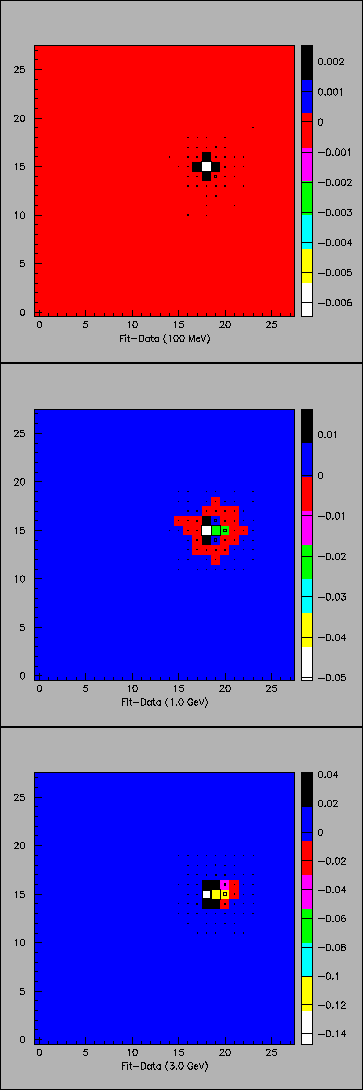 |
When is fixed to its average value of 1.7, the negative energy bias in
the fitted energy increases to
 . Comparing data with function,
block by block (Fig. 2), it is found that the negative bias comes
from an under-estimate of the two central blocks.
There are two possible explanations: MC showers are not Gaussian, or
we are misinterpreting the "true" shape by sampling a function
at the center of the block.
The second consideration is based on the following observation:
for radial widths of order
. Comparing data with function,
block by block (Fig. 2), it is found that the negative bias comes
from an under-estimate of the two central blocks.
There are two possible explanations: MC showers are not Gaussian, or
we are misinterpreting the "true" shape by sampling a function
at the center of the block.
The second consideration is based on the following observation:
for radial widths of order
 ,
a Gaussian is changing rapidly across the block.
While we sample the function at the center of the block, the actual function
value can be quite different at the block edges. It might be necessary to
integrate over a block to guess the shape of the PSF.
Proper normalization of the function requires multiplication with the block
area.
This is equivalent to 0-th order expansion of the integral
,
a Gaussian is changing rapidly across the block.
While we sample the function at the center of the block, the actual function
value can be quite different at the block edges. It might be necessary to
integrate over a block to guess the shape of the PSF.
Proper normalization of the function requires multiplication with the block
area.
This is equivalent to 0-th order expansion of the integral
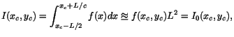 |
(4) |
around the center of the block  .
On the other hand, for any 2-dim function, a 2-nd order expansion can
be obtained from
.
On the other hand, for any 2-dim function, a 2-nd order expansion can
be obtained from
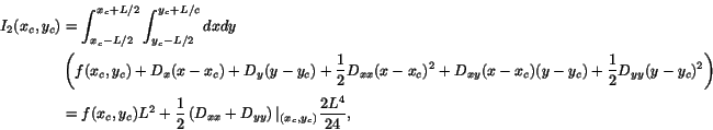 |
(5) |
where  stands for a partial derivative of
  with respect to a particular
index. In the case of the Gaussian, this is reduced to
with respect to a particular
index. In the case of the Gaussian, this is reduced to
 |
(6) |
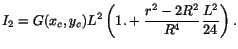
The true value of the integral over the block area is given by
![$\displaystyle I = \frac{E}{2} \left[ erf\left( \frac{\Delta x-L/2}{\sqrt{2}R} \...
...qrt{2}R} \right)
- erf \left( \frac{\Delta y+L/2}{\sqrt{2}R} \right) \right],$](img45.png) |
(7) |
with
 being
being
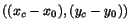 .
Table 1 shows a block-by-block comparison of data with
.
Table 1 shows a block-by-block comparison of data with
 ,
,  , and
, and  , from two showers with 1.0 GeV and 3.5 GeV photons.
For the first shower, the approximation is used as the PSF and the
radial width obtained is
, from two showers with 1.0 GeV and 3.5 GeV photons.
For the first shower, the approximation is used as the PSF and the
radial width obtained is
 if is allowed to vary.
One can see that significantly differs from and .
In the second case the integral is used as the PSF, with
if is allowed to vary.
One can see that significantly differs from and .
In the second case the integral is used as the PSF, with
 ,
where both and differ from .
,
where both and differ from .
Table 1:
Comparison between , , and from two fits.
Note: not all blocks with non-zero data have been shown.
 |
 |
 |
|
|
|
| 0.891053 |
19.606381 |
5.840514 |
1.607639 |
|
|
 |
 |
Data |
|
|
|
| 18.0 |
2.0 |
0.025080 |
0.030720 |
0.068005 |
0.065595 |
| 22.0 |
2.0 |
0.027360 |
0.016705 |
0.042231 |
0.044924 |
| 26.0 |
2.0 |
0.004560 |
0.000019 |
0.000112 |
0.000352 |
| 18.0 |
6.0 |
0.533520 |
0.530301 |
0.394643 |
0.408305 |
| 22.0 |
6.0 |
0.291840 |
0.288370 |
0.305232 |
0.279637 |
| 26.0 |
6.0 |
0.059280 |
0.000321 |
0.001467 |
0.002193 |
| 18.0 |
10.0 |
0.010260 |
0.018751 |
0.046285 |
0.046610 |
| 22.0 |
10.0 |
0.002280 |
0.010196 |
0.028374 |
0.031922 |
|
|
|
|
|
|
| 2.701281 |
21.084819 |
6.086944 |
0.966082 |
|
|
|
|
Data |
|
|
|
| 18.0 |
2.0 |
0.030780 |
0.000006 |
0.000115 |
0.005431 |
| 22.0 |
2.0 |
0.004560 |
0.000612 |
0.007948 |
0.036056 |
| 26.0 |
2.0 |
0.002280 |
0.000000 |
0.000000 |
0.000053 |
| 18.0 |
6.0 |
0.346560 |
0.044842 |
0.307623 |
0.339312 |
| 22.0 |
6.0 |
2.256060 |
4.686579 |
1.022599 |
2.252726 |
| 26.0 |
6.0 |
0.139080 |
0.000018 |
0.000317 |
0.003307 |
| 18.0 |
10.0 |
0.019380 |
0.000012 |
0.000229 |
0.008419 |
| 22.0 |
10.0 |
0.045600 |
0.001288 |
0.015373 |
0.055895 |
In Fig. 3
is shown the profile of the fitted energy as a function of
the generated energy obtained using . The energy bias is essentially
unchanged, relative to the case where is used.
The radial width again weakly depends on energy but it drops to
 averaged over photon energies. Table 2 shows
the average fitted as a function of shower energy.
Figs. 4, 5, and 6 show a comparison between MC data
and the PSF ( function), for fixed to the values from Table 2.
Comparing fit-data differences for various shower energies
(bottom right plots on Fig. 4, 5, and 6)
with the similar ones obtained by (Fig. 2) one can see
that central blocks are fitted better with than with .
averaged over photon energies. Table 2 shows
the average fitted as a function of shower energy.
Figs. 4, 5, and 6 show a comparison between MC data
and the PSF ( function), for fixed to the values from Table 2.
Comparing fit-data differences for various shower energies
(bottom right plots on Fig. 4, 5, and 6)
with the similar ones obtained by (Fig. 2) one can see
that central blocks are fitted better with than with .
Table 2:
Average and energies, and corresponding errors,
for fits obtained by the -function. Once is fixed to the value
from the left-most column, average fitted energy again decreases
so that overall negative bias reappears.
 [] [] |
[ ] ] |
 [] [] |
[] |
 [] [] |
[](fixed ) |
| 0.1 |
1.30 |
0.16 |
0.1 |
0.02 |
0.092 |
| 0.5 |
1.16 |
0.19 |
0.47 |
0.05 |
0.45 |
| 1.0 |
1.12 |
0.16 |
0.93 |
0.07 |
0.90 |
| 2.0 |
1.13 |
0.13 |
1.85 |
0.13 |
1.81 |
| 3.0 |
1.11 |
0.10 |
2.77 |
0.17 |
2.72 |
| 3.5 |
1.12 |
0.12 |
3.25 |
0.16 |
3.18 |
Figure:
The profile of the fitted energy as a function of the total energy
in the LGD, obtained using
 , and values of from the Table 2.
The straight dashed line represents unbiased fit.
, and values of from the Table 2.
The straight dashed line represents unbiased fit.
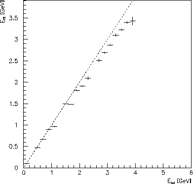 |
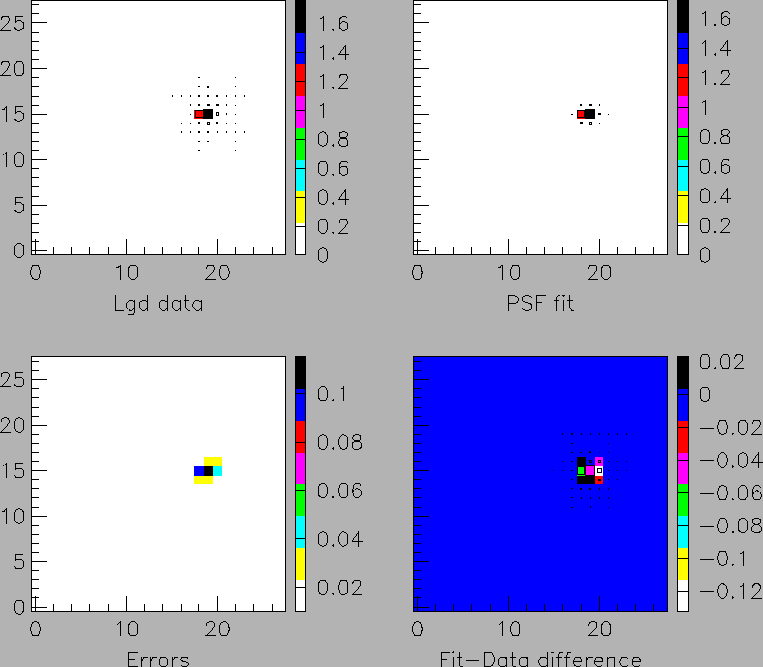
Figure 4:
Comparison of average data with
and PSF
(top-left and top-right plots respectively), for fixed ,
in the case of 0.1 GeV photons. Bottom-left plot represent errors,
while bottom-right shows fit-data difference. Box-plots are superimposed
for comparison.
 |
Figure 5:
The same as Fig. 4 for 1.0 GeV photons.
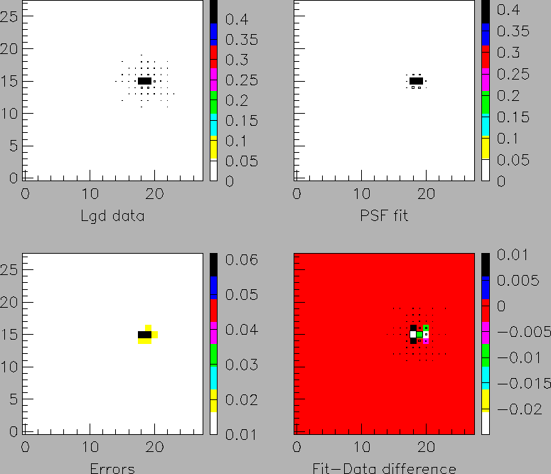 |
Figure 6:
The same as Fig. 4 for 3.5 GeV photons.
 |
Next: Discussion
Up: psf
Previous: Introduction
Richard T. Jones
2004-04-30