 |
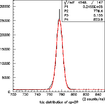
From Fig. 16 it is clear that to make further progress in reducing our electronics dead-time we have no choice but to compromise on our original wish for a online clean neutral trigger. The tdc spectrum for the CPV OR is shown in Fig. 18, taken during a run where the CP veto was removed from the trigger. All of the events in this sample passed the level 2 trigger condition. This figure shows that a veto window of 15ns is necessary in order to reject CP events online with full efficiency. Examination of the spectra for the individual counters shows that this peak width is essentially all coming from intrinsic time spread of the CP signals in the individual counters and not from timing misalignment.
There is no absolute reason why the CP veto must be done online.
Several have suggested that we could reduce the width of the online
CP veto window and accept a certain fraction of the CP events, and
then reject them offline using the tdc data. The model presented
above can be generalized to cover this possibility, albeit at the
expense of some additional complication. Eq. 12 above takes
on its simple form because it is assumed that CP events are
completely rejected at all beam intensities (see Eqs. 6,
9). Relaxing this assumption turns the two
terms of Eq. 12 into the eight terms of Eq. 18.
Actually we have no reason to decrease the veto window width for the
UPV OR, the problem is with the CPV OR. Therefore let
![]() .
This gets rid of the last four lines of Eq. 18 and leaves only
.
This gets rid of the last four lines of Eq. 18 and leaves only
![]() and
and
![]() as additional inputs to
extend the range of applicability of the model to
as additional inputs to
extend the range of applicability of the model to ![]() ns. The
formula for
ns. The
formula for
![]() now becomes
now becomes
| (19) |
 |
 |
The input parameters for the model used to generate
Figs. 19-21 are listed in Table 2.3.
For some of the input values to the generalized model I had to make an
educated guess. For example,
![]() is measured directly in
a run with the UPV veto enabled but the CPV veto removed. It appears
that we did not take any data under these conditions. By looking at
data with both CPV and UPV vetoes disabled, it is possible to check
how many of the events come with a coincident UPV signal and subtract
them off, but most of that data sample is completely skewed by the presence
of the level 2 trigger condition. Taking what I believe to be reasonable
estimates for the inputs that cannot be directly extracted from the data,
it is now possible to produce a realistic prediction for the yield of
signal events on tape as a function of
is measured directly in
a run with the UPV veto enabled but the CPV veto removed. It appears
that we did not take any data under these conditions. By looking at
data with both CPV and UPV vetoes disabled, it is possible to check
how many of the events come with a coincident UPV signal and subtract
them off, but most of that data sample is completely skewed by the presence
of the level 2 trigger condition. Taking what I believe to be reasonable
estimates for the inputs that cannot be directly extracted from the data,
it is now possible to produce a realistic prediction for the yield of
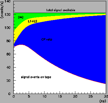
signal events on tape as a function of ![]() all the way down to zero
CPV window width. The result is shown in Fig. 19. The
conclusion from this plot is that the best yield is obtained with no
online CPV veto at all!
all the way down to zero
CPV window width. The result is shown in Fig. 19. The
conclusion from this plot is that the best yield is obtained with no
online CPV veto at all!
| parameter | value | method | |||||
|
|
/s/nA | fit to scaler data | |||||
|
|
/s/nA | fit to scaler data | |||||
| /s/nA | fit to scaler data | ||||||
| /s/nA | fit to scaler data | ||||||
|
|
s | to be chosen | |||||
|
|
s | to be chosen | |||||
| s | no CPV in trigger | ||||||
|
|
s | measured with UPV OR tdc | |||||
|
|
s | fit to scaler data | |||||
|
|
s | fit to scaler data | |||||
|
|
s | fast-clear specifications | |||||
|
|
s | measured on scope | |||||
|
|
s | promised by DAQ gurus | |||||
|
|
|
measured at low rate | |||||
|
|
|
measured with veto in/out | |||||
|
|
|
pure guess (should be small) | |||||
|
|
|
reasonable guess | |||||
|
|
1.0 | conservative estimate | |||||
|
|
|
reasonable guess | |||||
|
|
1.0 | conservative estimate | |||||
|
|
|
reasonable guess | |||||
|
|
|
fit to scaler data | |||||
|
|
|
fit to scaler data | |||||
|
|
|
reasonable guess | |||||
|
|
|
reasonable guess | |||||
The fact that we are writing all of this signal to tape does not necessarily
mean that it will be possible to recover offline the set of events with
accidental CPV hits within the coincidence peak. However the CPV is
highly segmented, which makes it possible to recover events with a CPV
inside the coincidence region provided that it does not physically
overlap with a cluster in the LGD. Hence the expectation is that many
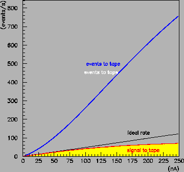
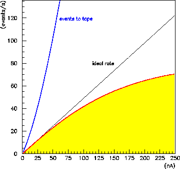
of these events will in fact be usable. Fixing ![]() , the yield
of signal events to tape under 1999 conditions, as a function of beam
current, is shown in Figs. 20-21. These two are the same
figure shown with different vertical scales. It is true that most of
the 800 events/s being written to tape at 250nA have charged particles in
the forward region. Most of them could be eliminated during a crude
one-pass reduction made offline. The most important conclusion of this
report is that only by disabling the online CPV veto can Radphi make
effective use of 250nA of beam, that corresponds to
, the yield
of signal events to tape under 1999 conditions, as a function of beam
current, is shown in Figs. 20-21. These two are the same
figure shown with different vertical scales. It is true that most of
the 800 events/s being written to tape at 250nA have charged particles in
the forward region. Most of them could be eliminated during a crude
one-pass reduction made offline. The most important conclusion of this
report is that only by disabling the online CPV veto can Radphi make
effective use of 250nA of beam, that corresponds to ![]() tagged photons/s.
tagged photons/s.