The charged particle veto wall is the component of Radphi that
encounters the highest rate, and so is the most sensitive part
of our apparatus to dead-time effects. It is important, therefore
that the model correctly describe the behavior of the logic that
generates the CPV OR. Similar to the UPV logic, the CPV OR is
formed by discriminating the individual signals from the 29
phototubes, producing for each a train of logic pulses of fixed
duration and then OR'ing these signals together. The formulae
which embody the model are as follows.
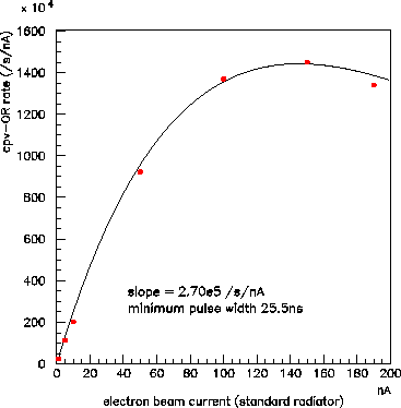
The results of a scan taken towards the beginning of the June period
is shown in Fig. 7. The tendency of the CPV OR scaler to
decrease at high rates is due to the fact that the scaler is counting
the transitions between 0 and 1 in the CPV OR signal and not the
amount of time it is on or off. At very high rates one expects the
scaler to go to zero (the CPV OR is always 1) which is the limit of
Eq. 8 at high rates. The two-parameter fit to the data
in Fig. 7 gives a fairly precise value of 25.5ns for ![]() ,
which disagrees with the value of 10ns that was programmed into the
OR module for its gate width. Upon examination, it was discovered that
the discriminator modules had been operating in updating mode, which
extends the width of the CPV OR signal to however long the pulse
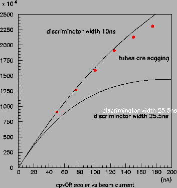
remains over threshold. A later scan shown in Fig. 8 gives
a more consistent value of 10ns for
,
which disagrees with the value of 10ns that was programmed into the
OR module for its gate width. Upon examination, it was discovered that
the discriminator modules had been operating in updating mode, which
extends the width of the CPV OR signal to however long the pulse
remains over threshold. A later scan shown in Fig. 8 gives
a more consistent value of 10ns for ![]() , indicating that the
problem was fixed. Once more the model correctly diagnosed a subtle
bug in the electronics and produced consistent results after the bug
was fixed.
, indicating that the
problem was fixed. Once more the model correctly diagnosed a subtle
bug in the electronics and produced consistent results after the bug
was fixed.
There are still significant deviations from the expected model behavior for the high-rate points in Fig. 8. One possibility is that it is due to CLAS emptying their target during that scan. A slight effect due to this is observable in these data: compare the U-shaped nonlinearity in the low-rate points in Fig. 6 with the corresponding points in Fig. 8. However the suppression at high rates goes beyond what would be expected based upon a comparison between those two figures (the data were taken during the same scan). The observation that the adc spectra from the central CPV counters showed a marked decrease in gain for the high-rate points taken during this scan indicates that some of the CPV tubes are showing signs of saturation.
The most important restriction on the validity of this model arises from
its ignoring the effects of discriminator dead-time at the level of
the individual counters. All of the observations made above under
the tagger section apply here as well. Because the rates in the
individual channels are limited to a few MHz, dead-time effects are
much less important there than they are once one is working with the
OR signal. Nevertheless losses at the level of 5% can be expected
from this source for those tubes running at 5MHz under full design
intensity. In order to take these losses into account consistently,
one must also bring in the two-pulse resolving power of these tubes
and electronics, which must be measured. At present the stability
of the beam current measurement is not sufficient to measure dead-time
effects a level better than 5%. In the present model they are being
ignored (set to zero). The restriction ![]() ns discussed
under the UPV section above also applies here as a condition for the
validity of Eq. 9
ns discussed
under the UPV section above also applies here as a condition for the
validity of Eq. 9