the level 0 trigger

Figure 9: Level 0 scaler rate vs. beam current measured at the beginning of the June run period.

Figure 10: Level 0 scaler rate vs. beam current measured at the end of the June run period.

The level 0 trigger is what generates the gate for the adc and tdc modules. The logic formula embodied in our present level 0 circuit is as follows.

$$L_0\;=\;\mbox{RPD}\;\cap\;\mbox{TAG}\;\cap\; \overline{\left( \mbox{CPV}\,\cup\,\mbox{UPV} \right)}$$ (11)

With the above calibrated model for the constituent signals, it should be possible to generate a prediction for the level 0 trigger rate. However there is some additional information that still must be supplied as input to the model, that is, the fraction of the total RPD OR rate that comes from trues $\cap$ Umiss $\cap$ Cmiss events. Let the intersection of Umiss and Cmiss sets be called noCP and the intersection of the trues and noCP sets be called signal. Not all signal events are interesting from the physical point of view, but they are the fish that this trigger has been designed to catch. Under conditions of low beam intensity, only signal events produce level 0 triggers. At high rates two things happen: signal events are lost, and non-signal events are picked up. Presumably higher level triggers and offline analysis will be able to discard the non-signal events, or at least subtract them away statistically, but the lost signal is a more serious problem; those events are gone forever. Let $f_n$ designate the fraction of the RPD OR rate that is noCP and let $f_s$ represent the fraction that is signal. Then

$$S_{_0} = r_{_R}\,I\,f_s\ {\cal F}_{true} (1-{\cal F}_{Umiss})\,(1-{\cal F}_{Cmiss}) +$$ (12)

$$r_{_R}\,I\ (f_n-f_s){\cal F}_{acc.} (1-{\cal F}_{Umiss})\,(1-{\cal F}_{Cmiss})$$

$$R_{_0} = \frac{S_{_0}}{1+S_{_0}(d_2+{\cal F}_2\,d_{_{DAQ}})}$$ (13)

where $S_{_0}$ is the rate observed in a free-running scaler monitoring the level 0 logic signal and $R_{_0}$ is the rate of level 0 triggers after the level 0 signal has been gated by the busy signal. The busy signal is present during level 2 processing (duration $d_2$) and during event readout (duration $d_{_{DAQ}}$) for events passed by level 2. The fraction ${\cal F}_2$ of level 0 triggers that are passed by level 2 is defined in the next section. The input parameters in the model are always represented by lower-case letters.

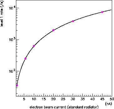
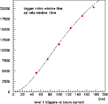
A comparison between the model and observations of $S_{_0}$ made towards the beginning and the end of the June period is shown in Fig. 9 and 10, respectively. Fig. 10 shows how complicated the shape is over the range of the scan. The linear region at low current transitions around 10nA to a quadratic behavior due to accidental coincidence with the tagger. Then above 50nA the quadratic rise stops and the curve turns over as the accidental charged-particle vetoes begin to suppress the trigger rate. The parameters that control the shape of this curve are $t_{_T}$, $t_{_C}$, $f_n$ and $f_s$; the first two were varied to fit the measured $S_{_0}$ data whereas $f_s$ and $f_n$ were measured independently during runs taken with special triggers. The agreement between the values for $t_{_T}$ and $t_{_C}$ with what is seen on the oscilloscope indicates that the electronics is behaving as expected. Note that $t_{_T}$ is expected to be a few ns less than the tagger OR pulse width because a few ns of overlap with the RPD OR signal is required before a coincidence is registered. Likewise $t_{_C}$ should be few ns less than the sum of the CPV OR and RPD OR pulse widths because only a few ns of overlap between the two is sufficient to generate a veto. This implies a practical minimum value on the effective veto window width of 8-10ns given that one is working with a minimum width around 5ns for the CPV OR and RPD OR signals.

The only new restriction that appears in the model at this level is that Eq. 12 implicitly assumes that the UPV OR and CPV OR signals are statistically independent. This is the assumption behind the factorization of the accidental veto probability into the product $(1-{\cal F}_{Umiss})(1-{\cal F}_{Cmiss})$. These two signals are certainly not independent because many tracks passing through the UPV will also create a signal in the CPV. However the UPV OR rate is so low that it makes very little practical difference how random UPV vetoes are accounted for in the model. At the other extreme one could assume that every UPV OR hit is accompanied by a CPV OR signal, in which case the factor $(1-{\cal F}_{Umiss})$ in Eq. 12 should be replaced by unity. At the full operating intensity of 250nA this increases the value of $S_{_0}$ by roughly 2%.