Certainly not everything in this Monte Carlo model is an accurate description of the Radphi calorimeter. The spectral attenuation of lead glass depends on its history and is almost certainly different for inner and outer blocks. The wrapping probably has air gaps in some places and none in others, which means that neither the black paper nor the aluminum foil models are really exact. Thus some checks are needed that the simulation gets the overall detector response right in regions where we already know the answer, before we can rely on it for guidance in the large-angle region where the response is unknown.
In the forward region ![]() we already know how the shower
depth
we already know how the shower
depth ![]() and yield
and yield ![]() should depend on photon energy
should depend on photon energy ![]() . Up
to an overall shift,
. Up
to an overall shift, ![]() should be proportional to the radiation
length times
should be proportional to the radiation
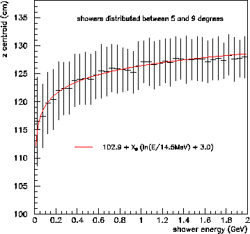
length times ![]() . The simulation data are shown in
Fig. 3 where only showers at
. The simulation data are shown in
Fig. 3 where only showers at ![]() have
been included. Superimposed on the data are two curves,
Eq. 5 in blue and the 2d parameterization in red. The
two curves are difficult to distinguish at the resolution of this
figure. This just reflects the fact that the depth calculation
under the new parameterization is just the same as Eq. 5
in the forward region. Fig. 2 shows that
have
been included. Superimposed on the data are two curves,
Eq. 5 in blue and the 2d parameterization in red. The
two curves are difficult to distinguish at the resolution of this
figure. This just reflects the fact that the depth calculation
under the new parameterization is just the same as Eq. 5
in the forward region. Fig. 2 shows that ![]() continues smoothly from this region to smaller values at higher
angles, partly from the geometric factor
continues smoothly from this region to smaller values at higher
angles, partly from the geometric factor ![]() and partly
due to shower leakage.
and partly
due to shower leakage.
 |
 |
 |
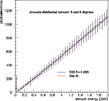
In the forward region we also already know that the curve ![]() vs
vs ![]() should look like Eq. 1. The simulation data are
shown in Fig. 4 where only showers at
should look like Eq. 1. The simulation data are
shown in Fig. 4 where only showers at
![]() have been included. Superimposed on the data are
two curves, a free fit to Eq. 1 in blue and the 2d
parameterization in red. Note that the free fit gives a value
of
have been included. Superimposed on the data are
two curves, a free fit to Eq. 1 in blue and the 2d
parameterization in red. Note that the free fit gives a value
of
![]() , to be compared with a value of 0.06 that
was obtained by D. Armstrong directly from Radphi data. The
agreement between the red and the blue curves shows that the
two embody essentially the same nonlinearity correction. Note
that this was not put into the simulation by hand. It emerged
from the interplay of internal reflection and attenuation effects
on the one hand, and leakage effects on the other. At large
angles one would expect leakage effects to win out over attenuation
and cause the sign of
, to be compared with a value of 0.06 that
was obtained by D. Armstrong directly from Radphi data. The
agreement between the red and the blue curves shows that the
two embody essentially the same nonlinearity correction. Note
that this was not put into the simulation by hand. It emerged
from the interplay of internal reflection and attenuation effects
on the one hand, and leakage effects on the other. At large
angles one would expect leakage effects to win out over attenuation
and cause the sign of ![]() to reverse. That is exactly
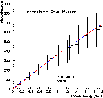
what the simulation shows. In Fig. 5 is shown
the same thing as Fig. 4 except that showers are
selected in the angular range
to reverse. That is exactly
what the simulation shows. In Fig. 5 is shown
the same thing as Fig. 4 except that showers are
selected in the angular range ![]() . Here the free
power-law fit gives an exponent less than 1. Again good agreement
is obtained between the fit to Eq. 1 and the 2d
parameterization.
. Here the free
power-law fit gives an exponent less than 1. Again good agreement
is obtained between the fit to Eq. 1 and the 2d
parameterization.
In conclusion, the new parameterization will reproduce the present known corrections to shower depth and energy for showers at low polar angle. In addition, it will give us reliable guidance for obtaining corrected values of these variables for large-angle showers. In the remaining section of this report a procedure is presented for how Eq. 2-4 may be solved in analysis code.