In Ref. [3] a detailed Monte Carlo simulation of the LGD
was described, based upon GEANT-3.21. The simulation tracks all
shower particles down to a kinetic energy of 100KeV, where they
stop emitting Cerenkov light and are stopped. The Cerenkov
light is then propagated down the block, undergoing reflections
until it is either absorbed or exits the block and is absorbed. Just
downstream of the block is a phototube; those Cerenkov photons
that are transmit into the glass surface of the phototube are
evaluated according to the quantum efficiency of the tube at the
given wavelength, and either discarded or counted in the
photoelectron sum ![]() . The measured attenuation spectrum of
clean lead glass is used by the simulation inside the block. Rays
that strike the surface of the block are stochastically transmitted
or reflected according to the familiar Fresnel formulae.
. The measured attenuation spectrum of
clean lead glass is used by the simulation inside the block. Rays
that strike the surface of the block are stochastically transmitted
or reflected according to the familiar Fresnel formulae.
The latter requires the knowledge of how the blocks are wrapped. In Ref. [3] I assumed that the block is surrounded by a layer of air followed by a non-reflecting surface. This permits total internal reflection at large incidence angles, but discards all photons that exit the glass. Under these conditions it was seen that the mean emission depth of the light observed at the phototube is not appreciably shifted by the presence of attenuation.
To check the sensitivity of this result to the wrapping, this study was
repeated [4] with an alternative wrapping model. In this
second model, the air gap was removed and a reflecting surface put in
its place with a reflectivity of 90%. As described in that report,
this change did make a noticeable difference, shifting the effective
shower centroid deeper into the glass by about 2cm, independent of
shower energy. Believing that this second model is a better approximation
to the actual LGD than the former, I update Eq. 3 of Ref. [3]
to read
To go beyond the restriction of normal incidence, a new simulation was
performed. In this simulation the reflective wrapping model was used
for the LGD. Photons were generated uniformly in energy from 0 to
2GeV. Runs of 1000 showers each were generated starting at
![]() up to
up to ![]() in steps of
in steps of ![]() . Each gamma ray
was independently tracked from inside the target to when all of its
energy was either absorbed or it exited the alcove area. All
phototubes were summed for each event, i.e. there was no clustering
performed, but only the blocks right around the shower core contributed
appreciably to the
. Each gamma ray
was independently tracked from inside the target to when all of its
energy was either absorbed or it exited the alcove area. All
phototubes were summed for each event, i.e. there was no clustering
performed, but only the blocks right around the shower core contributed
appreciably to the ![]() sum. For each detected Cerenkov photon
a record was kept of the
sum. For each detected Cerenkov photon
a record was kept of the ![]() coordinate where it originated, for
purposes of calculating the third coordinate of the shower centroid.
coordinate where it originated, for
purposes of calculating the third coordinate of the shower centroid.
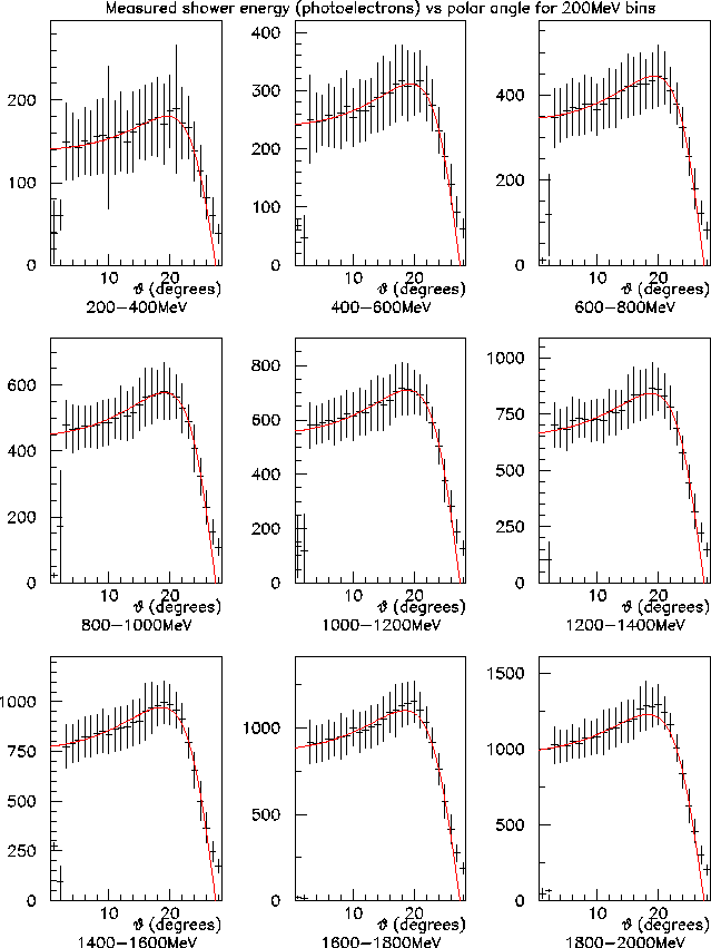
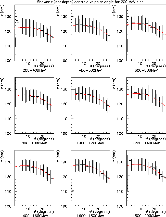
The showers were then binned in ![]() and
and ![]() , and the quantity
, and the quantity
![]() and the mean
and the mean ![]() were histogrammed on this grid. The results
can be seen in Figs. 1-2. The error
bars in these figures represent the r.m.s. fluctuations in those quantities
from one shower to the next; the error on the mean value itself is
about a factor of 30 smaller.
were histogrammed on this grid. The results
can be seen in Figs. 1-2. The error
bars in these figures represent the r.m.s. fluctuations in those quantities
from one shower to the next; the error on the mean value itself is
about a factor of 30 smaller.
 |
 |
In Fig. 1 one sees at all energies the expected decrease in
the observed yield that appears beyond ![]() . There are
a couple of interesting things to note here. First, the transition
from rising to falling gain does not show a kink, as would be obtained
if one just calculated the geometrical wall thickness along the photon
ray. This is because showers fan out as they develop and are not
confined to the ray of the original photon. Even more interesting is
the observation that the best energy resolution is obtained in a narrow
angular band around
. There are
a couple of interesting things to note here. First, the transition
from rising to falling gain does not show a kink, as would be obtained
if one just calculated the geometrical wall thickness along the photon
ray. This is because showers fan out as they develop and are not
confined to the ray of the original photon. Even more interesting is
the observation that the best energy resolution is obtained in a narrow
angular band around ![]() . This is seen in the figure at all
photon energies: the shortest %-error is obtained in the region just
beyond the turnover. This is the effect described by S. Teige (see previous
section) where at a certain block length there is a magic point where
the effects of attenuation and shower leakage tend to cancel and shower
conversion depth fluctuations do not affect the observed yield to
leading order. It is interesting to see how dramatic that effect is
in the simulation results.
. This is seen in the figure at all
photon energies: the shortest %-error is obtained in the region just
beyond the turnover. This is the effect described by S. Teige (see previous
section) where at a certain block length there is a magic point where
the effects of attenuation and shower leakage tend to cancel and shower
conversion depth fluctuations do not affect the observed yield to
leading order. It is interesting to see how dramatic that effect is
in the simulation results.
The corresponding results for ![]() are shown in Fig. 2.
Here the decrease at
are shown in Fig. 2.
Here the decrease at ![]() is less abrupt, but the effect is
clearly visible. One might be surprised to see that the mean depth
does not equal the front face of the glass at
is less abrupt, but the effect is
clearly visible. One might be surprised to see that the mean depth
does not equal the front face of the glass at ![]() . If one looks
at the Cerenkov
. If one looks
at the Cerenkov ![]() distribution for these showers, one sees a
sharp peak near the front of the glass corresponding to the shower
core, but then a tail extending downstream into the glass. This
tail comes from shower fragments that happen to split off the core
up near the front and move down into the block. As can be seen from
Fig. 1, only a fragment of the shower is visible to
the detector so there is a bias towards the part you can see.
distribution for these showers, one sees a
sharp peak near the front of the glass corresponding to the shower
core, but then a tail extending downstream into the glass. This
tail comes from shower fragments that happen to split off the core
up near the front and move down into the block. As can be seen from
Fig. 1, only a fragment of the shower is visible to
the detector so there is a bias towards the part you can see.
Overall these results are quite encouraging. They show that we
obtain a fairly good energy resolution all the way out to ![]() and perhaps further. However to make effective use of the these
high-angle showers we need to apply a
and perhaps further. However to make effective use of the these
high-angle showers we need to apply a ![]() -dependent gain
correction. The fits shown by the curves in
Figs. 1-2 are parameterizations of these
two-dimensional functions that will enable us to apply this correction
to our data.
-dependent gain
correction. The fits shown by the curves in
Figs. 1-2 are parameterizations of these
two-dimensional functions that will enable us to apply this correction
to our data.