Heating Unit Controls
Oscilloscope LabVIEW Program
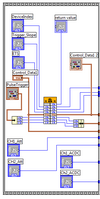
Frame 1:
Variables Used-
• DeviceIndex • Trigger_Slope • ETS • Control_Data1 • PulseTrigger
Functions-
• Unbundle – takes the values in a cluster and returns separate elements within the cluster as 1-dimensional values
• Bundle - takes multiple 1-dimensional values and combines them into a cluster
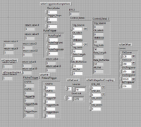
• Library Function* “sdSetTriggerAndSampleRate” – sets up a trigger to initialize other functions in the program as well as the time interval of data acquisition.
- (Note: The library functions are .DLL files and it requires decoders, usually in C++. Therefore, it is not quite possible to see exactly what the function is doing, but if the parameters fit the success criteria the output is either a 1 for success or 0 for failure. The inputs of the library functions are also preserved.)
Frame 2:
Variables Used-
• FiltAndTrigger • DeviceIndex • Control_Data1
Functions-
• Unbundle
• Library Function “sdSetFilt” – sets channel and filter trigger
Frame 3:
Variables Used-
• Device Index • Level • CH1_Att • CH2_Att • Ch1_ACDC • Ch2_ACDC • Control_Data1
Functions-
• Library Function “sdGetLevel” – reads waveform position adjust data from the oscilloscope
• Library Function “sdSetVoltageAndCoupling” – sets voltage and coupling of both channels of the oscilloscope
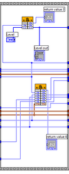
Frame 4:
Variables Used-
• DeviceIndex • Level
Functions-
• Library Function “sdGetLevel”
Frame 5:
Variables Used-
• Levers • DeviceIndex • CH1_Att • CH2_Att • PulseTrigger (unbundled) • Level
Functions-
• Library Function “sdSetOffset” – adjusts the position of the channel
Frame 6:
Variables Used-
• DeviceIndex
Functions-
• Library Function “sdCaptureStart” – starts to capture data from the oscilloscope
Frame 7:
Variables Used-
• DeviceIndex
Functions-
• Library Function “sdTriggerEnabled” – sets the trigger
Frame 8:
Variables Used-
• CH1_Voltage • CH2_Voltage • CH1_Att • CH2_Att • DeviceIndex • Ch1_ACDC • Ch2_ACDC • Control_Data1 • Pulse_Trigger • Level • Ch1Lever • Ch2Lever • Ch1TrigLever • Ch2TrigLever • TIMEBASE • ETS • Data_tab_ch1 • Data_tab:ch2 • X Minimum • X Maximum • Y Minimum • Y Maximum • Length
Functions-
• Bundle
• Unbundle
• Build Array – creates a multidimensional array from building multiple 1-dimensional arrays.
• Subset Array – creates an array of the length of all the input indices
• Write to Binary File – writes the data of the program to a file
• Waveform graph – creates a graph with plots from an input array.
• Library Function “sdGetData” – reads data from the oscilloscope
• Library Function “sdSetFilt”
• Library Function “sdSetTriggerAndSampleRate”
• Library Function “sdSetOffset”
• Library Function “sdSetVoltageAndCoupling”
Function of the Program:
Frames 1-7 of the LabVIEW program for the oscilloscope are part a flat sequence structure. It was most likely set up like this for organization and to ensure all of the functions and subVIs fire in the correct order. The first 7 frames are for initializing the data acquisition and the 8th fame has the bulk of the program functionality.
Frame 8:
The majority of Frame 8 is immersed in a “while” loop, which continues unless stopped. The first half of the “while” loop is inside of a case structure which is enabled or disabled by the push of a Boolean push-button; by disabling this case-structure, it makes the program run faster because there is no need to process data that need not be inputted. A case structure is wired to the CH1_Voltage variable; the case structure has a numeric value inside which changes to whatever the CH1_Voltage is equal to. Another case structure is set up in the same manner but the variable is for channel 2 (CH2_Voltage). CH1_Voltage and CH2_Voltage are compared to CH1_Att and CH2_Att respectively; if the channels’ voltages are not equal to each other, a Boolean value of true is produced and sent to an “or” comparator. The “or” comparator sends a value of true or false to another case structure which when “true,” sets voltages and couplings via the function “sdSetVoltageAndCoupling,” otherwise when false, funnels the CH1_Voltage and CH2_Voltage straight through. Concurrently, Ch1Lever, Ch2Lever, Ch1TrigLever, and Ch2TrigLever are bundled with the “Lever” cluster to create a larger cluster. This cluster with the CH1_Voltage, CH2_Voltage, DeviceIndex, Trigger Source, and Level are put into the Library Function “sdSetOffset.” From this, Trig_Source and TIMEBASE are bundled with Control_Data1 into a cluster. Most of the data is then wired into another flat sequence structure for two frames; Pulse_Trigger is unbundled into 1-dimensional arrays and wired to the function “sdSetTriggerAndSampleRate” along with DeviceIndex, TriggerSlope, ETS, and the bundled TIMEBASE and Trig_Source. The data is then moved to the second frame in this sequence where the DeviceIndex and FiltAndTrigger are put into the function “sdSetFilt.”
The last part of “initialization” is the funneling of all of the variables listed including data_tab_ch1 and data_tab_ch2, and a constant 0 into the “sdGetData” function, which sends the appropriate data to show on the waveform graph. This last half of the “while” loop has a sequence of case structures that may be disabled via use of push-buttons. If the return value of the “sdGetData” function has a successful value of 1 it then enables the next case-structure. The data from channel 1 of the oscilloscope then wired to two separate case-structures, one which is sent to a “write to file” function and the other to a graphing function. The case-structure which contains the “write to file” function can be enabled or disabled by a switch; the data is wired to an “array subset” function with the “length” as the length of the subset array and the “X Minimum” is the index. The last portion of the work of the program deals with the case-structure which contains the graphing function. The data from channels 1 and 2 are into a build array function and put into a “waveform graph” function, which can also be enabled or disabled via button. The data of the program is then put into a shift-register, which preserves the data and reuses it as starting values at the beginning of the register.
There are a couple other things in the program that are shown but do not quite pertain to the actual data acquisition. The scales of “X” and “Y” of the graph are depicted in the LabVIEW program. And, a trigger rate is shown; the trigger rate gives a value in hertz which shows how quickly the program is executing. For the most part, the more parts of the program enabled, the faster it runs. The controls enabler and the graph display take up the most processing power.


