Attenuation of light along BSD paddles

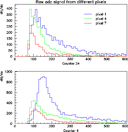
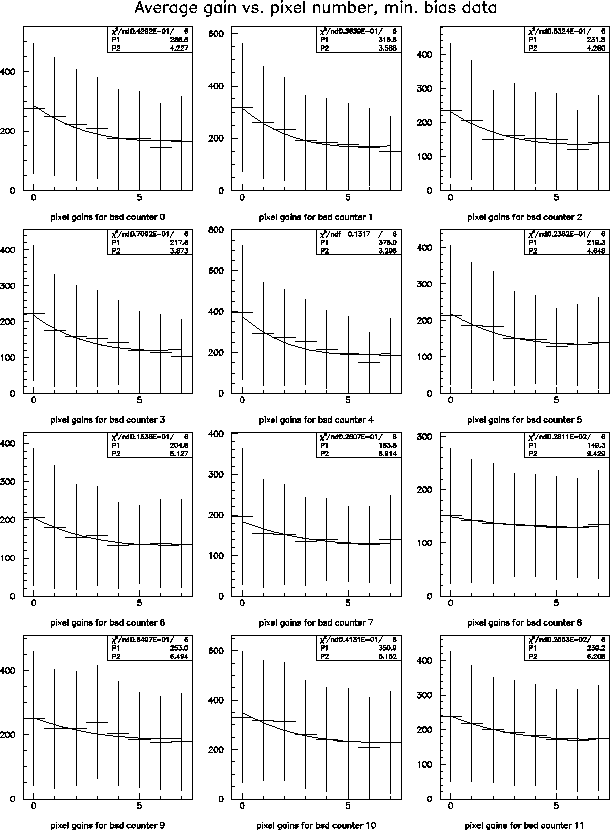
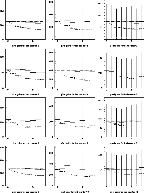
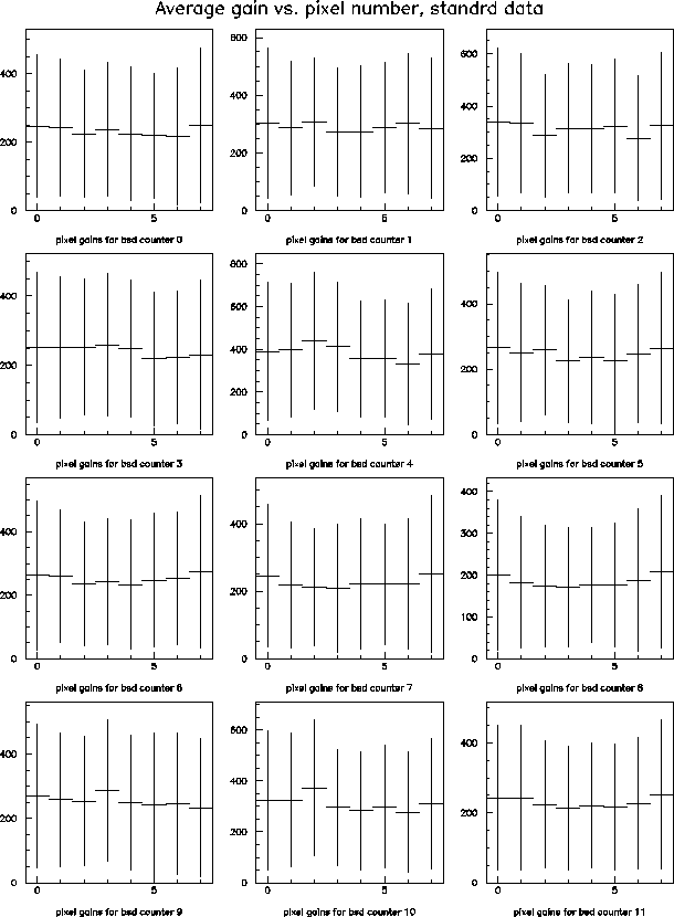
The adc signal from a BSD counter is proportional to the amount of collected light, or in other words to the deposited energy. When one compares different pixels in a given counter, it can be seen that peak position shifts toward lower values for higher pixel index (see Fig 2). The reason for that might be polar angle energy dependence or attenuation of light along the BSD counters. Since the same dependence is observed in both minimum-bias and standard data, it is concluded that attenuation of light is responsible for the observed gain dependence on pixel index. If the effect were due to the dependence of the particle spectrum on polar angle, the gain vs. pixel curve should be different for hadronic (standard) and electromagnetic (minimum-bias) backgrounds.

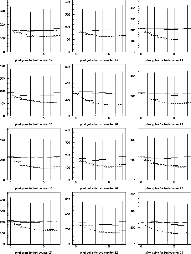
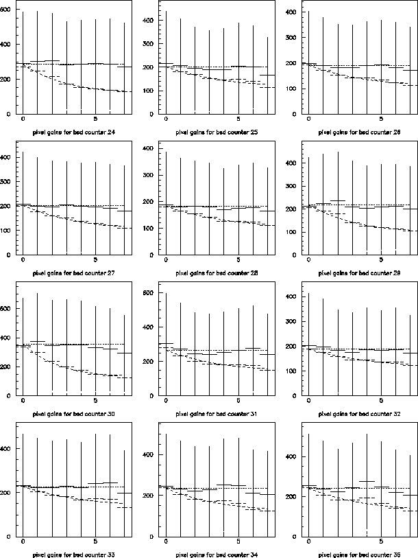
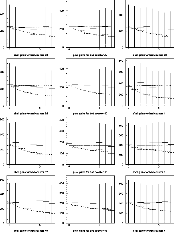
In order to explore this dependence, the distribution of mean adc gain as a function of pixel number is formed for every BSD counter. All distributions of pixel gains show the same characteristics (see Fig. 3): fast exponential drop for the first three pixels and a rather flat tail at higher pixels. An exponential drop would be expected from attenuation, while flattening might be due to reflection from the end of the counter. Thus, the sum of one falling and one increasing exponential function could be used to describe the data

$${g(z) \sim [exp(-bz) + C \, exp (bz)],}$$ (4)

where z is given in pixel units. The constant b is inversely proportional to the attenuation length while C takes care of the reflection coefficient and length of the paddle. Alternatively, one might explain the flattening of the gain curve at smaller angles by the increasing path length of the particle passing through the counter

$gain \sim L = a/sin(\theta) \sim \sqrt{r^2+z^2}$,

where a is the thickness of a paddle, $\theta$ is the angle from the beam axis ( $\theta \sim 30^{0}$ near the end of the detector), and r is the radius of a given layer. Taking into account these effects leads to following equation

$$g(z) = A \sqrt{r^2+z^2} [ exp(-z/B) + C exp(z/B) ].$$ (5)

This function has three parameters A, B, and C, where B is now proportional to the attenuation length. By fitting the distributions of pixel gains using this function with three free parameters it is possible to obtain good agreement with the data. However, it is found that a fit of equal quality can be obtained using a simpler function that is the sum of a falling exponential and a linearly increasing function (see Fig 3)

$$g(z) = A [ exp(-z/B) + Cz ].$$ (6)

This parametrization is found to yield parameters with smaller fluctuations from counter to counter than are obtained using Eq. 5. In Table 2 are given results of three and two-parameter fits, as well as average and r.m.s values of fitting parameters for the two different types of BSD paddles. After the fit, the parameter A is discarded since it can be absorbed into the gain. One can see that there are more variations of B for three than for two-parameter fit, and even negative values of C in the case of three-parameter fit. When parameter C is kept fixed (one value for spirals and one for straights), similar values of B are obtained for all BSD counters within particular layer. Because of the similarity of the pixel gain distributions from standard and minimum-bias data, and the larger statistics of standard data, we decided to take standard data to obtain the calibration constants,

$$cor(z) = \frac{g(0)}{g(z)} = \frac{1}{exp(-z/B) + Cz}.$$ (7)

Values of B and C used to correct pixel gains are given in the last two columns of Table 2. and they are obtained using standard run r8003. In Figs. 4 - 7 are shown pixel gain distributions, before (dashed crosses) and after corrections for attenuation (solid crosses) for all 48 BSD counters. As an example of how the attenuation correction procedure is checked, in Fig. 8 is given the pixel gain distribution of the first layer of BSD counters from the standard run r8600. The calibration constants were obtained from run r8003.

Figure 2: Raw adc signal from counters S24 and R04 for several chosen pixels, minimum-bias data.

Figure 3: Pixel gain distributions for the first layer of BSD counters (channels R0-R11). Solid lines represent the best fit obtained with three free parameters.

Table 2: Attenuation of light in the BSD counters: the best fit results in the case of three and two fitting parameters. The normalization parameter A is discarded.

			Minimum-bias data								Standard data
			Three parameters				Two par.				Two par.
	Counters		B				C				B				C (fix.)		B				C (fix.)
	R00		5.93				.034				4.23				.055		4.33				.057
	R01		4.74				.038				3.58						3.85
	R02		4.49				.054				4.27						4.01
	R03		6.80				.020				3.87						3.49
	R04		4.85				.029				3.29						3.12
	R05		5.58				.046				4.64						4.87
	R06		4.64				.063				5.13						4.17
	R07		4.44				.073				5.91						4.42
	R08		7.87				.066				9.42						5.98
	R09		15.67				.008				6.49						4.49
	R10		7.57				.032				5.15						3.72
	R11		5.95				.059				6.21						5.06
	L12		10.99				.026				6.26						5.83
	L13		7.54				.051				6.74						5.33
	L14		5.75				.058				5.88						3.69
	L15		5.77				.071				7.36						5.19
	L16		3.45				.062				3.77						2.97
	L17		4.35				.065				5.02						3.99
	L18		3.69				.068				4.49						3.81
	L19		5.59				.062				6.24						5.12
	L20		7.76				.033				5.19						4.64
	L21		6.63				.044				5.40						4.74
	L22		5.89				.029				3.96						3.97
	L23		9.81				-.001				3.95						3.49
	average/rms		6.49		2.61		.05		.02		5.27		1.4				4.35		0.8
	S24		4.88				.048				5.88				0.035		4.16				.037
	S25		16.91				.015				10.50						8.03
	S26		19.81				.003				9.25						7.42
	S27		11.23				.021				8.18						6.45
	S28		20.86				.001				9.38						7.67
	S29		6.12				.039				6.31						5.09
	S30		4.26				.041				4.59						3.60
	S31		5.79				.049				7.33						6.65
	S32		14.22				.018				9.67						8.69
	S33		43.43				-.021				9.17						7.67
	S34		47.81				-.036				7.35						6.36
	S35		48.22				-.029				8.31						6.54
	S36		23.32				-.012				7.83						6.87
	S37		8.64				.031				7.66						5.97
	S38		21.97				-.030				5.84						6.49
	S39		19.88				-.025				5.79						5.74
	S40		31.65				-.030				6.86						6.56
	S41		6.14				.014				4.32						3.54
	S42		12.74				-.007				5.74						4.73
	S43		22.98				.001				9.91						6.96
	S44		19.45				.013				11.24						6.23
	S45		8.80				.019				6.47						4.35
	S46		11.21				.034				10.33						7.77
	S47		8.65				.038				8.84						6.07
	average/rms		18.28		12.76		.008		.02		7.79		1.89				6.24		1.4

In conclusion, the analog signal from the BSD detector is analysed. It is observed that all BSD paddles have similar adc distributions. However, because of different characteristics of the counters, the position of the maximum varies from counter to counter. In order to correct for this, relative gain constants are found so that integrated spectra are matched to one chosen reference counter. In addition, it is seen that average gain depends on pixel position. Average gain decreases exponentially as pixel index increases, independent of the trigger type. Comparing standard and minimum-bias data it is concluded that the observed gain dependence comes from the attenuation of light along the BSD paddle. The gain dependence on pixel index is best described by a superposition of one falling exponential and one increasing linear function. Fit to the pixel gain distributions yields coefficients that can be used to correct for attenuation losses. These coefficients have similar values for different BSD counters.

Figure 4: Pixel gain distributions for channels R0-R11 after attenuation corrections. Dashed crosses represent gains before corrections. The dashed line represents the best fit obtained by use of Eq. 6 when C is kept fixed (see Table 2). The dotted line represents the expected gain level following the attenuation correction.

Figure 5: The same as Fig. 4 but for the left counters L12 -L23.

Figure 6: The same as Fig. 4 but for the straight counters S24 -S35.

Figure 7: The same as Fig. 4 but for the straight counters S36 -S48.

Figure 8: Standard run r8600: pixel gain distributions for channels R0-R11 after attenuation corrections performed using correction factors given in the last two columns of Table 2.