What we call the tagger OR is a logical OR of the 19 discriminators
monitoring the left-side phototubes on the top 19 tagger focal plane
paddles. Each input to the OR generates an edge-triggered internal
pulse of fixed duration; these are continuously OR'ed together to produce
a single signal that we call the tagger OR. Note that this is different
from what CLAS calls the tagger OR. The pulse duration is manually
adjustable in the tagger electronics racks. In this model it is currently
ignored (set to zero). The parameters in the model that concern the tagger
are the linear slope ![]() of the tagger OR in counts per nA, the tagging
coincidence window width
of the tagger OR in counts per nA, the tagging
coincidence window width ![]() and the scaler dead time
and the scaler dead time ![]() . The linear
slope is the proportionality constant between beam current and the
tagger OR rate in the linear region at low intensities.
. The linear
slope is the proportionality constant between beam current and the
tagger OR rate in the linear region at low intensities.
In the model, every signal in the Radphi detector arises either from the interaction of a tagged photon (or its prompt reaction products) or it does not. These two are called trues and accidentals in the following discussion. By a tagged photon is meant a bremsstrahlung photon that was generated in the same electromagnetic cascade that contained an electron which produced a pulse over discriminator threshold in the left side of one of the tagger focal plane counters. The distinction between trues and accidentals is in the physics of the event that caused them, not in the temporal proximity of the tagger and detector signals, although the above restriction to prompt reaction products excludes trues where the two signals are separated by hundreds of nanoseconds. At finite rates it is practically impossible to distinguish trues from accidentals on an event-by-event basis. Nevertheless, as long as the events are independent, the two categories of events are distinct from each other and can be treated as two separate populations, to be added together in the end.
The content of the model is embodied in the following three formulae.
The parameters ![]() and
and ![]() were extracted from a two-parameter fit
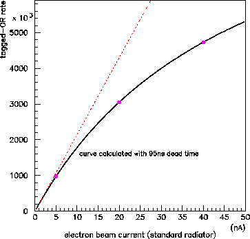
of measured tagger OR rates vs. beam current taken during the June
run. The results from a scan taken early in the run are shown in
Fig. 1. The dotted line shows the linear extrapolation with
were extracted from a two-parameter fit
of measured tagger OR rates vs. beam current taken during the June
run. The results from a scan taken early in the run are shown in
Fig. 1. The dotted line shows the linear extrapolation with
![]() from low rates. The saturation of the measurements gives a value
for the scaler dead time
from low rates. The saturation of the measurements gives a value
for the scaler dead time ![]() of
of ![]() ns. This large dead time is
completely out of line with the specification for the scaler (200MHz),
and indicates that there is an additional dead time hidden somewhere
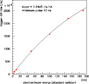
in the system that is not in the model. It turned out that the tagger
discriminator widths had not been properly set. When this was done,
a new scan produced the data shown in Fig. 2, now shown all
the way out to 200nA. A new fit yields 10ns for
ns. This large dead time is
completely out of line with the specification for the scaler (200MHz),
and indicates that there is an additional dead time hidden somewhere
in the system that is not in the model. It turned out that the tagger
discriminator widths had not been properly set. When this was done,
a new scan produced the data shown in Fig. 2, now shown all
the way out to 200nA. A new fit yields 10ns for ![]() , which is in
good agreement with the width of the tagger OR pulse width seen on the
oscilloscope. Although the model is merely descriptive at this point,
getting reasonable values for the parameters provides a good check that
the electronics is working as expected.
, which is in
good agreement with the width of the tagger OR pulse width seen on the
oscilloscope. Although the model is merely descriptive at this point,
getting reasonable values for the parameters provides a good check that
the electronics is working as expected.