the current situation

Figure 15: Decomposition of signal losses among various stages of the event pipeline as a function of the width of the CPV veto window $t_{_C}$ at a beam intensity close to the maximum point in the scan taken at the end of the June period. Values of $t_{_C}$ below 15ns represent an extrapolation of the model beyond its range of validity because in that regime the CP vetoes cannot be treated as fully efficient.

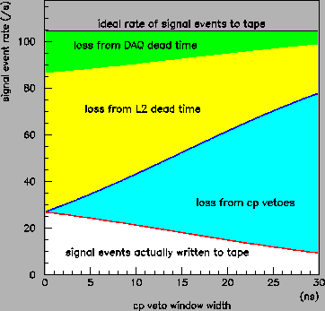
Supposing then that the model is giving correct results, what part of the electronics chain is producing the majority of the losses? The answer to this question is illustrated in Fig. 15. Depending upon what value one takes for the width of the CP veto window, the losses are shared more or less equally between random CP vetoes and dead-time associated with the level 2 processor, with data acquisition contributing an additional 10-15%. Recall that there is a restriction on the validity of the model that $t_{_C}\ge 15$ns. Reducing $t_{_C}$ below this bound will introduce a leak in the CP veto and cause the losses from the level 2 processor and DAQ to increase faster with decreasing veto window width than is shown in the plot. Fig. 15 actually includes extra losses at level 2 from some broken adc channels that generated significant processing overhead during the June period, which explains why this figure looks somewhat worse than the situation at 250nA in Fig. 12 where the broken channels have been removed. Nevertheless the conclusion from this figure is correct that the CP veto and the level 2 processor are primarily responsible for the losses in our present setup.

Table 1: Parameters supplied as input to the model, together with information about how the value for the parameter was obtained.

	parameter		value		method
	$r_{_T}$		$1.94\cdot 10^5$		/s/nA		fit to scaler data
	$r_{_R}$		$1.45\cdot 10^3$		/s/nA		fit to scaler data
	$r_{_U}$		$1.4\cdot 10^4$		/s/nA		fit to scaler data
	$r_{_C}$		$2.7\cdot 10^5$		/s/nA		fit to scaler data
	$t_{_T}$		$1.4\cdot 10^{-8}$		s		fit to scaler data
	$t_{_C}$		$1.2\cdot 10^{-8}$		s		fit to scaler data
	$d_{_T}$		$1.0\cdot 10^{-8}$		s		fit to scaler data
	$d_{_C}$		$1.0\cdot 10^{-8}$		s		fit to scaler data
	$d_2$		$1.4\cdot 10^{-5}$		s		measured on scope
	$d_{_{DAQ}}$		$6.7\cdot 10^{-4}$		s		measured on scope
	$f_s$		$2.6\cdot 10^{-3}$				measured at low rates
	$f_n$		$5.5\cdot 10^{-1}$				measured with veto in/out
	$f_{2s}$		$1.3\cdot 10^{-1}$				fit to scaler data
	$f_{2n}$		$3.5\cdot 10^{-3}$				fit to scaler data

A complete list of the model inputs used to generate the figures in this section is given in Table 2.1. Many of these numbers changed as timing, thresholds and gains were adjusted throughout the run period. A few were sensitive to the quality of the beam tune. The numbers given in the table are the ones that describe the situation during the intensity scan taken at the end of the June period.