yield of all-neutral hadronic events

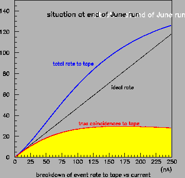
Figure 12: Comparison between ideal and actual rates of recording signal events on tape as a function of beam intensity, evaluated by the model under the conditions at the end of the June 1998 run period.

As has been shown in the previous sections, the model gives a good description of the full set of counting rates of relevance to our trigger from very low intensities up to the beam current at which Radphi has been designed to operate. The model now permits a decomposition of the event sample collected at any given beam intensity into signal and background components, and to compare the efficiency for signal collection at various beam currents. 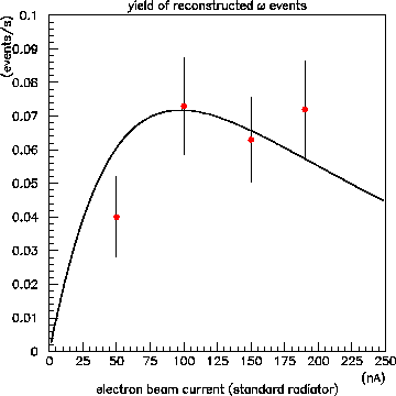The rate at which signal events are recorded on tape, denoted $S_{_S}$, is given by

$$S_{_S} = r_{_R}\,I\,f_s\ {\cal F}_{true} (1-{\cal F}_{Umiss}... ...{\cal F}_{Cmiss}) \,f_{2s}\,\left(\frac{R_{_0}}{S_{_0}}\right)$$ (15)

which is to be compared with the corresponding rate for an experiment without any dead-time effects, $S_{_I}$,

$$S_{_I} = r_{_R}\,I\,f_s\,f_{2s}$$ (16)

which is directly proportional to the beam intensity. The situation at the end of the June period is summarized in Fig. 12. In particular, it shows that increasing the beam current above 100nA does very little to increase the rate at which signal is being written to tape; in fact above 175nA it begins to decrease. Given that the proposal assumed no dead-time effects and an intensity that corresponds to 250nA on this figure, we are presently a factor of 4 short of our design goal in terms of rate capability.

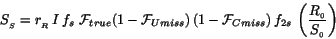
Figure 13: Comparison between ideal and actual rates of recording signal events on tape as a function of beam intensity, evaluated by the model under the conditions at the end of the June 1998 run period.

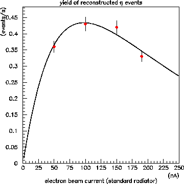Figure 14: Comparison between ideal and actual rates of recording signal events on tape as a function of beam intensity, evaluated by the model under the conditions at the end of the June 1998 run period.

Given that no single stage of the electronics or data acquisition chain was operating near its maximum rate (the phototubes and bases on the CPV were running near their limit but they do not contribute dead-time within this model) there is good reason to be skeptical that the overall losses are so high. As a check on this result, Scott Teige analyzed the data from the intensity scan taken at the end of the June period, and extracted the yield of $\eta$ and $\omega$ mesons from their $2\gamma$ and $3\gamma$ decays respectively. The yields are plotted as a real-time rate in Figs. 13-14. The solid curves are the shape of the signal (red) curve from Fig. 12. Fig. 13 in particular gives striking confirmation of the model prediction.