RTJ's  PWA Logbook
started May 20, 1999
last updated Nov 15, 2000
The partial wave analysis of the Jetset
data sample has been carried out in
collaboration by Antimo and me. I was responsible for laying the
theoretical groundwork and producing the amplitude generator, and Antimo
carried out the fits. The summary of Antimo's work and discussions with
collaborators regarding his results can be found
here. Before
we go to press with our results, we thought it would be best to do a
cross-check of each others' work. This logbook summarizes the results
of my own independent pwa that I am carrying out as a part of this
cross-check. It is not meant to be exhaustive, but rather to be as quick
as possible. We just want to be sure that the major conclusions of our
paper survive an independent analysis. The event selection criteria are
not being examined. Rather, I obtained the event sample for this analysis
directly from Antimo, so we can be sure we are working from the same data.
This applies both to experimental data and to Monte Carlo. We are sharing
the same subroutine that generates the partial wave amplitudes, that I
wrote some time ago, and cross-checked again during the month of March.
Other than that, we are not sharing analysis tools.
- Which waves need to be included in the fit?
- Do we agree on the normalization integrals?
- Are we using the same resonance lineshape for the
phi?
- How do we know when we have a good fit?
- How can we relate the fit parameters of AP to those used
by RJ?
- How do the results compare with the total cross section
we published?
- Do we have evidence for a resonance at 2.230?
Which waves need to be included in the fit?
[RTJ] May 20, 1999-
Total spin S
 must be
equal for the two waves. This turns out to be the same as the statement
that two waves of opposite parity cannot interfere. This rule follows
from the fact that our initial state is unpolarized.
must be
equal for the two waves. This turns out to be the same as the statement
that two waves of opposite parity cannot interfere. This rule follows
from the fact that our initial state is unpolarized.
- If J=0 for one of the waves then the other wave must have J=even. This follows from the general properties of Clebsh-Gordon coefficients.
The somewhat arbitrary rule that we adopted when we started the PWA was
that we would include all allowed waves up to and including J=4 and
L = 4 (G-wave) where
L is the orbital
angular momentum of the
final state. The list of all allowed waves under this restriction is
shown in Table 3 taken from an earlier
draft of the PWA article.
= 4 (G-wave) where
L is the orbital
angular momentum of the
final state. The list of all allowed waves under this restriction is
shown in Table 3 taken from an earlier
draft of the PWA article.
The symmetries of the strong interaction of the
final state have been very useful in reducing the total number of
waves we need to include in the pwa to these 23. The symmetries
further simplify the problem by reducing the number of interference
terms that contribute to the differential cross section. Cross terms
between two waves in the amplitude sum are zero unless the two waves
satisfy both of the following criteria.
In order for the fit to return a reliable error estimate on the parameters it is important that the waves supplied as input be linearly independent. This means that not only must they be mathematically different functions but their orthogonality must survive to some approximation after the experimental acceptance is applied. The partial wave sum has been constructed out of a set of orthogonal functions. This means that when integrated over angles all of the cross terms vanish. This guarantees that the functions are linearly independent, that is, that the angular distribution corresponding to a given set of amplitudes is unique, up to the well-defined set of ambiguities discussed above. This statement is only rigorously correct in the case of unit acceptance.
To see how the
orthogonality of the above waves survives the acceptance, I used the full
Monte Carlo sample of events generated according to
phase space to numerically integrate over angles every term in the pwa
sum. These numbers can be viewed as a matrix with one wave index labeling
the row and the other labeling the column. Each
element of the matrix was computed together with its error (from Monte
Carlo statistics) and is shown in Table 1. In
the case of unit acceptance this would have come out as the unit matrix,
within errors. Note that the waves have been renormalized so that the
diagonal terms are unity. I did this to make it easy to evaluate the
effects of acceptance on the distinguishability of waves. If the acceptance
were uniform, the off-diagonal elements would be zero. If one of the
cross terms were unity, it would mean that those two waves are
indistinguishable given our acceptance. The fact that all of the cross
terms are at the level of 10% or smaller indicates that even with our
large acceptance corrections, from a statistical point of view our
apparatus is quite capable of telling all of these waves apart.
Of course systematics are the bugger.
A priori all of these waves are important. I see no reason why any of them can be eliminated from the fit by general arguments or why any of pair of them should be considered redundant. According to our Monte Carlo, they are all distinguishable even after acceptance is applied.
Do we agree on the normalization integrals?
[RTJ] May 21, 1999The maximum likelihood method requires that the parameterized distribution that forms the hypothesis must be normalized. In general, the normalization is a function of the parametes, which means that the distribution function must be re-normalized at every step in the search. This is facilitated by calculating the integral over angles of each term in the sum-amplitude-squared before launching the fit, so that the normalization can be calculated as a simple quadratic sum over the parameters when the search is underway. These so-called normalization integrals have been calculated using the same Monte Carlo sample by both Antimo and me, and so comparing our results provides a useful check.
Antimo calculated the integrals from Monte Carlo for each of the 58 individual momentum settings in our data set, and then fitted them to a single polynomial function of pbar momentum. He sent me the code that evaulates these polynomials. In Fig. 1 I show my own calculated normalization integrals as data points with error bars (Monte Carlo statistical error) for each of the 58 runs. Superimposed on the data is the polynomial fit from Antimo. I have rescaled all of the integrals so that if the acceptance were uniform they would all be unity. These plots show which waves are favored or disfavored by our acceptance. There are corrections as large as a factor of 2, but none of the waves are lost.
Overall there is good agreement. However there are significant deviations in places. I believe that the deviations are mainly the consequence of trying to force a polynomial through a curve with rather non-analytic behaviour in places. Consider wave 6 for example. The deviations from the fit are as large as 40% in places. My choice is to use the Monte Carlo values themselves (the points in these plots) rather than a parametrization. The statistical errors on the points are small compared to the error one makes in trying to force a smooth curve through them. Apart from this procedural difference, it is clear from the figure that Antimo and I are working with the same normalization integrals.
I think there is some problem on some of the integrals. I have plotted my values with fits in the usual web page. They can also be found here 1-9, 10-18 and 19-23.
Yes, I have found the difference. In calculating my normalization integrals
I am including all solutions within a certain radius of the
peak in the
Monte Carlo Goldhaber plot, and then dividing by the total number of solutions.
You must be somehow taking just one solution per Monte Carlo event, and
then dividing by the number of
events generated. How do you chose which solution to count? The one that
lies closest to the
peak?
We agree at momenta above 1.5GeV because that there is only one solution
in the
region per event, so you get the same one no matter how
you chose it (count all hits within a given radius, chose the nearest
to the mass peak per event, or something else). What is happening at low
momenta is that 4K phase space has shrunk far enough that my circle around the
peak now
overlaps with the ridge of "reflection" solutions that lies along the upper
diagonal of all of the Goldhaber plots. The angular distribution of these
reflection solutions must be radically different from phase space in order
to drive some of these normalization integrals crazy as soon as they start
to get included in the integral.
In my opinion, we should stay away from the reflection region of the
Goldhaber plots in this analysis. Even at the lowest momentum there is a
clear dip between the
peak
and the reflection ridge. So what I have done is to decrease the size
of my circle around the
peak
for the lowest momentum points. My values for the mass cut radius are
given, together with the integrated luminosity, in
Table 2 for each data point in our sample.
The revised normalization integrals with these modified cut radii are
shown in Fig. 2. The agreement with Antimo's fits
is now excellent. I do still see regions where the fit deviates from the
Monte Carlo data by more than the statistical errors, and so I will continue
to use the MC data themselves instead of a fit. But from these plots it
is apparent that the normalization integrals cannot give rise to any
signficant disagreements between this work and that of Antimo.
The way the I have selected the solution is to take the one closest
to the
peak. Here is the slide as a PS file that
shows how this works.
I have no real reason to prefer my method of selecting solutions over yours, provided that we restrict ourselves to a region close enough to the peak to exclude reflections. We are now doing essentially the same thing to select our solutions. Now, on to the fit...
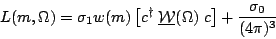
Are we using the same resonance lineshape for the phi?
[RTJ] June 6, 1999- Using channel likelihood weights for the function w(m) in
Eqn.5 already includes the information about the
fraction contained in the data sample. Including the variable parameter
x to adjust the signal/background fraction a second time
is redundantly redundant. It is absent from Eqn.7.
-
The w(m) function was formed by taking the ratio of B(m) / P(m)
and so should be represented by the ratio of weights w/w' if
channel likelihood weights are to be used to determine the shape of the
peak.
The shape of the peak in the Goldhaber plot is
purely empirical, being determined almost entirely by our experimental
resolution. The narrowness of the allows
us to use the narrow resonance approximation, in which the differential
cross section for
production factorizes into a mass part and an angular part as follows,
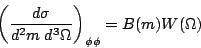 | (1) |

 ,
m
,
m
 and
and  to represent the 3 pairs of angles that
describe the final state. If one could isolate a pure sample of
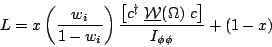
events then
the angular analysis would not depend on knowing the shape B(m).
However, all of our samples have some background mixed in with the
events, so what
we measure is actually
to represent the 3 pairs of angles that
describe the final state. If one could isolate a pure sample of
events then
the angular analysis would not depend on knowing the shape B(m).
However, all of our samples have some background mixed in with the
events, so what
we measure is actually
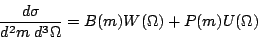 | (2) |
peak, i.e.
4K phase space is used to extrapolate the shape of the background from the
tails to the region inside the peak. For the shape of the background
angular distribution we have basically no guidance. Antimo has chosen to
use isotropic phase space, and I will continue with this choice for the
present time. The problem is that, while this is almost certainly wrong, it
is going to be hard to prove it wrong from our data because the statistics
in the wings of the peak are very poor. A corollary of this statement is that
if the deviation in the background from a uniform angular distribution cannot
be extracted from the data due to poor statistics then the statistical errors
from this analysis will be sufficient to cover this systematic. In the end
we will need to vary this shape somehow and report the sensitivity of our
results to this assumption as a contribution to our systematic error.
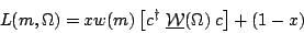
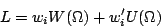
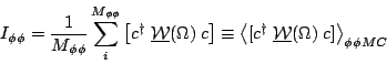
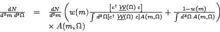
Our PWA code is written with the total cross section absorbed into the
the angular function W() in
Eq. 2 to form a differential cross section. This
can be written in compact matrix form in terms of the partial wave amplitudes
c as follows
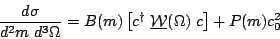 | (3) |
 parameterizes
the magnitude of the background and W()
is now a matrix of known angular functions that does not vary during the fit.
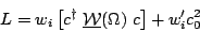
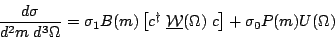
The expression in Eqn.3 above can be simplified for use
in a maximum likelihood fit by dividing out common factors that do not
depend on the fit coefficients. Dividing out P(m)
gives the (unnormalized) hypothesis,
or likelihood, for the measured distribution in mass-angle space
parameterizes
the magnitude of the background and W()
is now a matrix of known angular functions that does not vary during the fit.
The expression in Eqn.3 above can be simplified for use
in a maximum likelihood fit by dividing out common factors that do not
depend on the fit coefficients. Dividing out P(m)
gives the (unnormalized) hypothesis,
or likelihood, for the measured distribution in mass-angle space
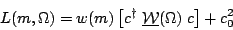 | (4) |
density B(m)
to phase space P(m) in the Goldhaber plot. This equation can by mapped
onto equation 5 of our draft pwa article as
 | (5) |
)
and defining parameter x = 1 /
(1 + c� )
which varies over the interval [0,1]. Since the likelihood gets normalized
after the acceptance is applied, a simple rescaling is OK, but I think there
is a problem with how this equation is being used in the analysis we describe
in the draft paper.
Whether one starts from (3) as I do, or (5) as Antimo does, should make
no difference, provided that we are using the same shape for the
peak w(m). Antimo is using the
weight factors from the channel likelihood analysis of the Goldhaber plot to
evaluate the w(m) factors for each event. Channel likelihood
gives three weight factors for each event: w, w', and w''
where w is the
weight, w' is that of non-resonant 4K, and for points where it
is important, w'' is that of KK.
These three factors sum to unity for each event. That means that if you make
three Goldhaber plots, each weighted with one of the w factors from
channel likelihood and then add them up, you should get back the original data.
That is, leaving aside KK for simplicity,
 | (6) |
peak.
This is not equivalent to Eqn.5 for two reasons.
I would recommend the following modified form for an analysis that uses
the channel likelihood weights to set the peak shape.
 | (7) |
I think you are right concerning the use of the weights from channel likelihood. In this way we also fix the phi phi contribution with respect to background. I presume the method is similar to your way of removing the background. I am repeating the fits using this method. Preliminary results show that the D0 amplitude gets larger and errors became smaller.
Can we compare directly the functions that we are using for the function
w(m)? It is a 2D function, but I have made a radial projection around
the central mass of the and then cut a slice
through the origin to show the shape of the peak. It is plotted in
Fig. 1. Note that because it is a ratio of two
distributions B(m) / P(m) both the shape and the normalization are
significant. We have to agree on this function if our fits are going to be
compared. Antimo, can you plot yours in a similar way, so we can compare them?
The way I obtained this shape was by taking the Monte Carlo
Goldhaber plot
and making a radial projection to reduce it to one dimension. I defined
the range of the radius such that it cut off before reaching the reflection
region of the Goldhaber plot. I normalized the MC data to have a unit integral
over the Goldhaber plot. This is my Monte Carlo estimator function for
B(m).
I then did the same for the 4K Monte Carlo, but this time I had to be very
careful about the normalization. 4K MC looks like a flat distribution over
the Goldhaber plot, but only because you have included all three solutions from
every event. Depending on how you chose your solutions, you can get very
non-uniform mass distributions for 4K. To keep things simple and smooth,
I included all solutions as a part of P(m) and normalized the 4K Monte
Carlo to 3 over the whole Goldhaber plot. This is my Monte Carlo estimator for
P(m).
In the end I only consider the region
centered around the peak, but in this way my normalization of P(m) is
consistent with that described above for B(m). I could have defined
P(m) as the distribution of only the nearest solution per event to
the
peak, and normalized to unity. This will give the same answer as
my method (it had better!) provided that the normalization integral for the
nearest-solution approach stays away from all of the reflection regions.
Since I do not know where all of the reflection areas from the lower-left
region lie, I decided my procedure was easier. It probably doesn't matter.
Anyway, since Antimo is using the nearest-solution approach, this alternative
approach gives us a cross check.
To obtain the function w(m) I first smooth the P(m) radial
plot by a polynomial fit, and then divide the B(m) plot by it. The
resulting Monte Carlo estimate for w(m) I then fit to a double-gaussian
with 4 parameters: two heights and two sigmas. The mean values are fixed at
the mass. This double-gaussian fit provides
an analytic function that gets evaluated for every event and provides the
values for w(m) that go into the likelihood.
Let's compare our w(m) functions and make sure we agree before we go on and do the angular distributions. I now have results for the partial wave analysis, by the way, but don't want to show anything until we have set up the problem in the same way and can make an intelligent comparison of our respective results.
I agree with the equations you are using. I have attached the plot you are asking for.
The scale and resolution of this plot make the shape of the peak hard to
read. I have plotted the same data, but with better resolution, for a
couple of points in our momentum scan. Here they are for
point 7 and point 10.
These data are the values of
w /
w' in the language
of Eqn.7. On these plots I have superimposed my weight
function w(m) from Eqn.3. With the higher
resolution in these plots, you can see several different trajectories.
These come from the different runs that were combined together to make
the one data point. They all have the same shape, but different normalizations
that reflect the different admixtures of background that channel
likelihood saw for each run. Variations of a factor of 2-3 like this
are reasonable between runs, seeing how the conditions of the trigger
(especially the Cerenkov) changed from year to year. By comparison,
my w(m) function has a fixed normalization that is derived from
Monte Carlo and the relative sizes of the background and signal contributions
to the Goldhaber plot are adjusted (parameter
c) during the pwa fit.
The comparison should address the shape only, and not the relative scale.
The conclusion from these two plots is that there is very little difference
between the my peak shape that Antimo is now using. We are making real
progress.
In the procedure I am following, both the
fraction
and the angular distribution parameters emerge from the same fit. So
the first check on the validity of the results is to look at the quality
of the fit on the mass spectra. This amounts to integrating over all
angles and plotting the distribution in masses. The fit only covers a
limited region of the Goldhaber plot that lies within a circle whose radius
varies with energy and is chosen to exclude the reflection band. The
results of the fit are shown in Table 4 below. The
corresponding results from channel likelihood, labeled as Antimo in the plot,
are also shown. Channel likelihood provides an analysis of the entire
Goldhaber plot and so the column labeled fit radius does not apply to
Antimo's results.
| point no. |
momentum range (MeV) |
integrated luminosity (/nb) |
fit radius (MeV) |
N (this work) |
N  (this work) |
N (Antimo) |
|---|---|---|---|---|---|---|
| 1 | 1180-1200 | 86.566 | 25 | 355 � 24 | 66 � 16 | 379 � 28 |
| 2 | 1220-1246 | 94.778 | 30 | 451 � 27 | 188 � 22 | 489 � 32 |
| 3 | 1260-1280 | 89.767 | 35 | 587 � 30 | 309 � 25 | 647 � 35 |
| 4 | 1300-1330 | 100.170 | 40 | 777 � 36 | 432 � 30 | 844 � 39 |
| 5 | 1345-1390 | 103.494 | 45 | 938 � 41 | 656 � 38 | 1006 � 42 |
| 6 | 1390-1404 | 94.122 | 50 | 1121 � 43 | 726 � 38 | 1241 � 46 |
| 7 | 1405-1430 | 104.093 | 55 | 1549 � 51 | 1119 � 47 | 1724 � 54 |
| 8 | 1435-1465 | 88.509 | 60 | 1217 � 47 | 1026 � 45 | 1321 � 48 |
| 9 | 1465-1500 | 80.625 | 60 | 1152 � 45 | 1043 � 44 | 1211 � 47 |
| 10 | 1505-1650 | 73.836 | 60 | 903 � 43 | 1096 � 45 | 860 � 42 |
| 11 | 1700-1800 | 70.218 | 60 | 668 � 32 | 1860 � 47 | 926 � 46 |
| 12 | 1900-2000 | 66.883 | 60 | 640 � 47 | 1733 � 57 | 739 � 42 |
-
The x and y phi-band plots showing the
quality of the fits can be seen by clicking on the underlined values
in the column labeled
N
) of phase
space times acceptance. Over most of the energy range of this experiment
the product is strikingly close to uniform across the Goldhaber plot. The
phi-band plots are only shown to suggest the quality of the agreement
between data and fit.
How do we know when we have a good fit?
[RTJ] August 25, 1999
By a good fit we mean one that is statistically compatible with the data.
With binned data the  � provides the
classic means for judging goodness of fit. In the case of our angular
distributions, however, binning the data is not appropriate. A single
measurement is represented by 6 angles (3 pairs): the production angles,
and the two sets of decay angles. One of these, the production azimuth,
can be discarded because of symmetry. Even so, if one were to divide each
axis up into 30 divisions, the full histogram would contain in excess of
24 million bins, most of whom would be empty. Reducing the number of
bins substantially would introduce a bias to our PWA by filtering out
waves in the data that vary more rapidly in angle than others. Thus we
need a method for judging goodness of fit that does not require binned
data, for which the classic choice is the likelihood ratio test.
� provides the
classic means for judging goodness of fit. In the case of our angular
distributions, however, binning the data is not appropriate. A single
measurement is represented by 6 angles (3 pairs): the production angles,
and the two sets of decay angles. One of these, the production azimuth,
can be discarded because of symmetry. Even so, if one were to divide each
axis up into 30 divisions, the full histogram would contain in excess of
24 million bins, most of whom would be empty. Reducing the number of
bins substantially would introduce a bias to our PWA by filtering out
waves in the data that vary more rapidly in angle than others. Thus we
need a method for judging goodness of fit that does not require binned
data, for which the classic choice is the likelihood ratio test.
The likelihood ratio test works as follows. Suppose one has a Monte
Carlo generator that generates according to a distribution controlled
by M parameters. He can then use this generator to create any
number of samples of a given size, each of which are statistically
consistent with the parent distribution, but independent of each other.
These samples can then be submitted to a fit, and maximum likelihood
estimates of the original parameters can be obtained for each sample
generated. For each sample one then has two numbers, L0 and
Lmax. Lmax is the value of the likelihood at the maximum,
the value that is returned from the fit. L0 is the value of the
likelihood for the sample if one calculates it using the true parameters
that were used by the generator. These two are different numbers because
the fit will prefer parameters slightly away from the true ones in the
general case for finite samples. It can been proved that the quantity
2ln(Lmax/L0) is distributed as a �
with M degrees of freedom. The conditions for this proof are fairly
general, but it is strictly only true in the limit of large sample size.
This test can be turned around to function as a goodness-of-fit test in the following way. The "true" values of the parameters (PWA amplitudes) are unknown to us. But the maximum likelihood test tells us that if a given set of parameters might be the true ones (statistically compatible) then the likelihood L0 must be close enough to Lmax to give a reasonable value for the log-ratio statistic given above.
First I want to test the MLT on Monte Carlo. To do this, I produced 100
different sets of initial PWA amplitudes, chosen at random. For each of
the 12 data points I then generated 100 Monte Carlo data sets, with similar
statistics in
and 4K events to what is shown in Table 4. In this
test we are looking for two deviations. The test statistic is expected to
behave like a � with M degrees
of freedom, 45 in the present case. If the test statistic comes out
systematically low then it means that the effective number of degrees of
freedom that are controlling the shape of the data is less than we think.
This is possible if, for example, the same or similar shape can be made
by different combinations of waves. Note that it is only events within
the acceptance of our apparatus that are contributing to the likelihood;
changes in the shape of the parent distribution that take place outside
the acceptance do not affect the likelihood analysis. On the other hand,
if the test statistic comes out systematically higher than expectation then
it means that there are systematic errors in the model that are biasing
the maximum likelihood fit away from the true parameters. One example of
such a systematic is detector angular resolution, whose effects are not
taken into account in our PWA model. Such problems are expected to show
up in the fits to Monte Carlo as well as in real data.
| point no. |
momentum range (MeV) |
N |
N |
N in |
N out |
2 ln(Lmax/L0) |
|---|---|---|---|---|---|---|
| 1 | 1180-1200 | 346 � 44 | 370 � 46 | 66 � 0 | 42 � 12 | 32 � 10 |
| 2 | 1220-1246 | 411 � 87 | 415 � 85 | 186 � 0 | 183 � 12 | 27 � 11 |
| 3 | 1260-1280 | 576 � 46 | 563 � 47 | 315 � 0 | 328 � 17 | 32 � 9 |
| 4 | 1300-1330 | 731 � 104 | 671 � 95 | 449 � 0 | 513 � 21 | 46 � 12 |
| 5 | 1345-1390 | 881 � 170 | 835 � 158 | 637 � 0 | 681 � 28 | 39 � 11 |
| 6 | 1390-1404 | 1072 � 122 | 970 � 113 | 740 � 0 | 840 � 27 | 56 � 13 |
| 7 | 1405-1430 | 1486 � 220 | 1366 � 202 | 1137 � 0 | 1261 � 41 | 66 � 11 |
| 8 | 1435-1465 | 1202 � 84 | 1062 � 84 | 1044 � 0 | 1179 � 34 | 63 � 14 |
| 9 | 1465-1500 | 1148 � 32 | 991 � 41 | 1063 � 0 | 1211 � 34 | 80 � 16 |
| 10 | 1505-1650 | 902 � 30 | 802 � 39 | 1101 � 0 | 1210 � 28 | 62 � 13 |
| 11 | 1700-1800 | 668 � 26 | 325 � 40 | 1414 � 0 | 1754 � 37 | 178 � 27 |
| 12 | 1900-2000 | 639 � 26 | 527 � 35 | 1223 � 0 | 1339 � 27 | 64 � 12 |
Point 11 is special because I was unable to obtain a Monte Carlo 4K sample
for one of the runs in that point, which throws off the normalization
integrals. The rest of the points look more reasonable. There is a bias
towards underestimating the
component that increases with energy. It is well known that the maximum
likelihood method carries some bias, so this is no surprise. For all
except the highest points the bias is 10% or less. It could be removed
by momentum-dependent tweaking of the resonance lineshape, or can be removed
by a post-fit correction. For the moment, I am not particularly interested
in tweaking things. Our major objective is to come to a conclusion
soon about the quality and uniqueness of the PWA solution being
proposed by Antimo.
I propose that we proceed in the following way. To judge the quality of
the fit, I would like to receive a set of PWA amplitudes from Antimo
from which I will calculate the likelihood. This likelihood I will
then compare with the maximum-likelihood Lmax that I get leaving
all of the waves free. From the ratio of the two likelihoods I will form
the above � statistic, and see if it
is consistent with being drawn from the distributions listed in the last
column of Table 5. If so, then I am satisfied with
the fit. We then need to decide how to talk about uniqueness in the paper.
Can we agree on this procedure?
If you go on my pwa web page you will find the information you asked for. In particular, the list of waves is explained in the text dated 26 May 1999. The amplitudes are (13,11,12,x,y) where x,y may change from one bin to the other and are written in the minuit output. The list of amplitudes is always in my JETSET NOTE 96-01.
-
Antimo has a strict cut around the
peak to select those solutions that
are admitted to the pwa. From the 1996 draft of the PWA paper he
records that only mass bins with over 50%
from channel likelihood are included.
I estimate that this results in a cut radius of about 20MeV around the
center of the
peak. For my analysis, I have drawn as large a
circle as I can have and still avoid the kinematic reflection band in
the Goldhaber plot. The radii I am using are shown in column 4 of
Table 4.
-
For the shape of the peak, Antimo is
using the weights from channel likelihood, whereas I am using a mass-
dependent fit to projections of the Goldhaber plot to a sum of two Gaussians.
- We use different ways of normalizing the angular distribution. Antimo fixes the amplitude of the leading wave to unity and then divides by the normalization integral at each point. I use the extended likelihood procedure. Extended likelihood treats all amplitudes as independent variables, but automatically constrains the total expected yield to equal the total number of observed events through the use of something like a Lagrange multiplier.
I found the results indicated above from Antimo here. Without changing anything, I simply copy the final amplitudes that Antimo has provided and plug them into my fit. I want to emphasise that this is an important test of the robustness of these results, because of the following differences between my and Antimo's approach.
and
background events. This is really orthogonal to what we are after
in this study, however, which is to determine the goodness-of-fit of the
angular distributions to the data. Hence any decrease in the likelihood
that I calculate for Antimo's fit parameters that comes from his shift
in the total
cross section away from my best-fit value should be removed before we do
the comparison. That way any likelihood decrease that is observed can be
associated with the angular fit alone.
Both of these things are actually easy to do. First I wrote a small
script to input Antimo's parameters from his results file and write
input data files in the format required for my fit function. Then I
fixed the angular amplitude coefficients in MINUIT and told it only to
treat the total yields of
and background events as fit variables.
Following this two-parameter fit, I come up with a new likelihood that
I call Antimo's likelihood. This can be compared directly with
my Lmax from the full 23-wave fit. The results are shown in
Table 6 below.
| point no. |
momentum range (MeV) |
N (full fit) |
N (full fit) |
N (Antimo) |
N (Antimo) |
2 ln(Lmax/L0) |
|---|---|---|---|---|---|---|
| 1 | 1180-1200 | 355 � 24 | 66 � 16 | 332 � 22 | 89 � 15 | 35.7 |
| 2 | 1220-1246 | 451 � 27 | 188 � 22 | 427 � 23 | 212 � 18 | 42.2 |
| 3 | 1260-1280 | 587 � 30 | 309 � 25 | 570 � 27 | 326 � 21 | 50.2 |
| 4 | 1300-1330 | 777 � 36 | 432 � 30 | 765 � 30 | 444 � 24 | 63.6 |
| 5 | 1345-1390 | 938 � 41 | 656 � 38 | 922 � 33 | 672 � 29 | 55.0 |
| 6 | 1390-1404 | 1121 � 43 | 726 � 38 | 1096 � 31 | 751 � 25 | 49.6 |
| 7 | 1405-1430 | 1549 � 51 | 1119 � 47 | 1511 � 37 | 1157 � 32 | 80.0 |
| 8 | 1435-1465 | 1217 � 47 | 1026 � 45 | 1175 � 32 | 1068 � 31 | 58.2 |
| 9 | 1465-1500 | 1152 � 45 | 1043 � 44 | 1105 � 30 | 1090 � 30 | 86.2 |
| 10 | 1505-1650 | 903 � 43 | 1096 � 45 | 854 � 26 | 1145 � 31 | 88.0 |
| 11 | 1700-1800 | 668 � 32 | 1860 � 47 | 643 � 16 | 1885 � 39 | 62.6 |
| 12 | 1900-2000 | 640 � 47 | 1733 � 57 | 576 � 16 | 1797 � 38 | 85.4 |
-
The full fit shown in Table 6 is the same as that
reported in Table 4.
It contains 23 waves plus one parameter for background for a total
of 45 degrees of freedom. Antimo's solution is restricted to 5 waves
per point, so it carries 11 degrees of freedom. This means that the
hypothesis entailed in Antimo's solution is equivalent to the statement
that the numbers in the last column are distributed as a
with 34 degrees of freedom. When compared with the last column in
Table 5, these data are in fair agreement with
the hypothesis.
The small errors reported for the resonant and non-resonant yields from Antimo's solution is a reflection of the fact that these were obtained from my own refit where I froze the angular distributions according to Antimo's solution but allowed the fit to reapportion the total yields, as I explained above. Freezing the angular distributions reduces the statistical errors on the yields because the errors do not include the statistical fluctuations coming from uncertainty in the detector acceptance that arises from errors in the angular distribution.
- a minimal set of waves that gives an acceptable fit
- the best-fit values for the amplitudes of the selected waves
Antimo's solution can be taken at two levels:
| point no. |
momentum range (MeV) |
-ln(Lmax) (full fit) | -ln(L0) (Antimo) | -ln(L5) (5-wave refit) | 2 ln(Lmax/L5) | correlation factor |
|---|---|---|---|---|---|---|
| 1 | 1180-1200 | 3239.9 | 3261.2 | 3254.2 | 28.6 | 0.978 |
| 2 | 1220-1246 | 4997.7 | 5021.3 | 5018.2 | 41.0 | 0.985 |
| 3 | 1260-1280 | 6851.0 | 6879.0 | 6875.9 | 49.8 | 0.990 |
| 4 | 1300-1330 | 8898.8 | 8933.5 | 8930.4 | 63.2 | 0.986 |
| 5 | 1345-1390 | 11842.4 | 11871.4 | 11866.1 | 47.4 | 0.984 |
| 6 | 1390-1404 | 12755.6 | 12783.5 | 12774.0 | 36.8 | 0.993 |
| 7 | 1405-1430 | 18297.1 | 18341.1 | 18319.3 | 44.4 | 0.988 |
| 8 | 1435-1465 | 15671.4 | 15702.8 | 15690.4 | 38.0 | 0.982 |
| 9 | 1465-1500 | 14897.9 | 14941.6 | 14922.9 | 50.0 | 0.988 |
| 10 | 1505-1650 | 13653.8 | 13697.9 | 13684.4 | 61.2 | 0.990 |
| 11 | 1700-1800 | 15948.2 | 15995.1 | 15974.8 | 53.2 | 0.968 |
| 12 | 1900-2000 | 14294.1 | 14334.7 | 14318.6 | 49.0 | 0.933 |
The hypothesis (a) above is sustained if the values in the next to last
column of Table 7 are compatible with a
with 34 degrees of freedom. I would argue that these data support the
hypothesis, but the matter should be discussed. The last column was
included to give an idea of how different the angular distributions
coming from the 5-wave refit are from those of Antimo. The correlation
is defined as the expectation value of
(xy - <x><y>)
where x
is the angular density function from Antimo's fit and y is the one
coming from my 5-wave refit. The expectation value is evaluated on
Monte
Carlo data. The high degree of correlation shows that, the two solutions
have essentially the same shape, at least over that part of phase space
where we have data. The agreement is impressive, in view of the fact
that we admit different events to the pwa, and gives us confidence that
the shapes we extract are not too sensitive to these kind of details.
How can we relate the fit parameters of AP to those used by RJ?
[RTJ] February 25, 2000
Antimo and I are working with the same data and Monte Carlo samples,
and are extracting the same information from the data, but we use
different approaches at numerous points. For example, Antimo accepts
only one mass combination per event for input to the PWA, the one closest
to the
point on the Goldhaber plot, whereas I accept all solutions within a
given radius of the peak.
Since the kinematic reflection of the resonant peak is far from the
region of the Goldhaber plot, this should not make much difference to
our
PWA, and consistency between our two approaches is a useful check of
the robustness of the analysis. Another difference is that Antimo
fits in the space of (modulus,phase) for each complex wave amplitude
in the pwa, whereas I fit in the space of (real,imaginary) parts of
the same parameters. The main difference comes in how the errors are
estimated when the modulus errors are large. Because of theses differences
it is important that we be able to compare the results from our two
methods, and show they are consistent. In Table 7
the large correlation factor (last column) shows that the shapes of the
angular distributions extracted from our two fits have similar shapes,
but this does not necessarily mean that our amplitude coefficients are
in agreement. One might have two angular functions that are close to
each other in the region of our acceptance, but which come from distant
points in parameter space. To check if our parameters are unique, we
need to compare the parameter values directly. Before that is possible,
we need to see how the likelihood parameterization used by Antimo
corresponds to the one I use.
The likelihood in use by Antimo is given in his online logbook entry [AP} 26-May-1999 as
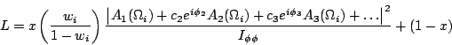 | (8) |
The expression in Eq. 8 is not written correctly, but I believe it is
coded correctly. What is wrong is that the amplitude squared written as
|A+...|
must be averaged over initial p,pbar spins outside the absolute value bars.
All of this is done correctly by the routine wave4K
that I wrote and both Antimo and I are using to generate the angular
distribution from the underlying amplitude coefficients, so I think
the error is only in the way the likelihood is written down. The correct
expression for the quantity returned by the function wave4K
is the one I wrote down in Eq. 3 above,
namely the trace [c W() c] where the full partial
wave angular information is encoded in the matrix
W()
of angular functions. In this case the matrix is of dimension 23�23.
The corrected expression for Antimo's likelihood is given in Eq. 9.
W() c] where the full partial
wave angular information is encoded in the matrix
W()
of angular functions. In this case the matrix is of dimension 23�23.
The corrected expression for Antimo's likelihood is given in Eq. 9.
 | (9) |
His normalization integral
I![]()
![]() is a function of the coefficients c given by
is a function of the coefficients c given by
 | (10) |
where the sum is over the events in the
Monte Carlo sample that passed all online and analysis cuts and
were reconstructed within the region of interest in the Goldhaber plot.
Note that in this form the likelihood is independent of the overall
scale of the c coefficients and so Antimo is free to choose
his normalization condition by setting
c=1 arbitrarily.
My own approach based on Eq. 3 treats the c coefficients as actual T-matrix elements, and so the likelihood does depend on the overall scale: it gives the total cross section. This enables me to fit the mass plot (do channel apportioning) and angular distributions all at the same time. While this has nice features, it makes a comparison with Antimo difficult because his fit assumes the Goldhaber plot has already been described by channel likelihood and fits only the angular part. Therefore I factor out the total cross section to a separate factor and impose a normalization condition on the angular part that fixes the overall scale of the c's. In this way, Eq. 3 becomes Eq. 11.
 | (11) |
Here B(m) and P(m) are the same normalized Goldhaber plot
densities from before, U() is uniform
in all center-of-mass angles (phase-space),
 is the total
cross section and
is the total 4K non-resonant cross section.
Both [c
W() c] and
U() are normalized to unity when
integrated over all six center-of-mass angles. This constraint, together
with a convention to fix the overall phase of the {c}, are
enforced using Lagrange multipliers. Dropping factors common to the
two terms in Eq. 11 and substituting for U()
gives the likelihood in Eq. 12.
is the total
cross section and
is the total 4K non-resonant cross section.
Both [c
W() c] and
U() are normalized to unity when
integrated over all six center-of-mass angles. This constraint, together
with a convention to fix the overall phase of the {c}, are
enforced using Lagrange multipliers. Dropping factors common to the
two terms in Eq. 11 and substituting for U()
gives the likelihood in Eq. 12.
 | (12) |
To see the correspondence between Eq. 9 and Eq. 12, we need the
relation between my function w(m) = B(m)/P(m) and Antimo's
weight
w from channel likelihood.
 | (13) |
where N![]()
![]() is the number of
events from channel likelihood and
N
is the number of
events from channel likelihood and
N is the number of background (non-resonant 4K) events in the Goldhaber plot.
Solving for w(m) gives Eq. 14.
is the number of background (non-resonant 4K) events in the Goldhaber plot.
Solving for w(m) gives Eq. 14.
 | (14) |
The correspondence is complete when we determine the meaning of the parameter x in Antimo's fit.
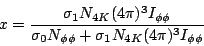 | (15) |
So x is a complicated parameter that can take on any value between
0 and 1.
Recall that I![]()
![]() is a function of the PWA amplitudes c, so x depends on
all of my parameters
,
and the c coefficients. It cannot be interpreted as the
fraction
of the sample, or anything simple like that.
However, when Antimo allows x to vary freely with c in his
fit he is effectively doing the same thing as I am doing when I vary
and
in my fit. In the end I can interpret
and
as total cross sections, whereas the fit value of x has no such
straight-forward meaning. However, since the PWA is concerned with the
c parameters only, I agree that there the two approaches are equivalent.
is a function of the PWA amplitudes c, so x depends on
all of my parameters
,
and the c coefficients. It cannot be interpreted as the
fraction
of the sample, or anything simple like that.
However, when Antimo allows x to vary freely with c in his
fit he is effectively doing the same thing as I am doing when I vary
and
in my fit. In the end I can interpret
and
as total cross sections, whereas the fit value of x has no such
straight-forward meaning. However, since the PWA is concerned with the
c parameters only, I agree that there the two approaches are equivalent.
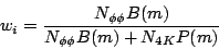
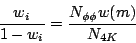
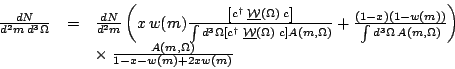
From values of x and the amplitudes c in my fit, how do
I calculate the
partial cross sections for each wave?
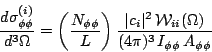
I take Eq. 9 as the starting point for deriving how a partial cross section comes out of Antimo's fit. To see how a cross section comes out of this, we need to start by remembering how the channel-likelihood weights are being used to partition the Goldhaber plot into resonant and non-resonant contributions as follows.
 | (16) |
The acceptance integrals in each denominator assure that integrating both
sides over angles gives an identity, and that the Ch.L. weights w
partition the events between
and
background. Comparison of Eq. 16 with
Eq. 9 shows a close resemblance, once you divide
out common factors and realize that the normalization integral
I![]()
![]() is just the ratio of the two denominator integrals in
Eq. 16. However there is a new parameter x in
Eq. 9 that must be introduced into
Eq. 16 to make the correspondence complete. The
complete form is shown in Eq. 17
is just the ratio of the two denominator integrals in
Eq. 16. However there is a new parameter x in
Eq. 9 that must be introduced into
Eq. 16 to make the correspondence complete. The
complete form is shown in Eq. 17
 | (17) |
This ugly extra factor
(1-x-w+2xw) is required so that integrating both sides over angles still gives back
the identity. What is the meaning of this x parameter? To see
that, we can use Eq. 17 to extract the total number of
in the
measured sample. First we integrate over angles and keep only the
term; the angular integrals in numerator and denominator cancel and leave
behind only the factors containing the mass dependence. Next we want
to integrate over masses to get a total count. Here we see that the
integral over dm with the factor
dN/dm in the integrand corresponds
to a simple sum over all of the events in the measured sample. This
result is given in Eq. 18
is required so that integrating both sides over angles still gives back
the identity. What is the meaning of this x parameter? To see
that, we can use Eq. 17 to extract the total number of
in the
measured sample. First we integrate over angles and keep only the
term; the angular integrals in numerator and denominator cancel and leave
behind only the factors containing the mass dependence. Next we want
to integrate over masses to get a total count. Here we see that the
integral over dm with the factor
dN/dm in the integrand corresponds
to a simple sum over all of the events in the measured sample. This
result is given in Eq. 18
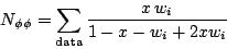 | (18) |
If x=0.5 then this expression reverts back to the standard formula
that N![]()
![]() is just the sum over the
measured sample of w.
This allows an interpretation of this mysterious factor x, that it
allows the PWA fit to make a correction to the Ch.L. apportioning if
it wants to. If the fit returns x=0.5 then the PWA agreed with
Ch.L. about how many
were in the sample. If the fit returns x>0.5 [<0.5] then it wants to
increase [decrease] the
fraction
over the Ch.L. value. This suggests that before proceeding to make cross
sections, you should check that the values of x coming back from
the fits make sense. Remember that the PWA fit is done over only a
restricted part of the Goldhaber plot, where it may not be easy for the
fit to tell resonant from non-resonant contributions. In that case it
may make sense to place some constraints on the allowed values
for x in the fit.
is just the sum over the
measured sample of w.
This allows an interpretation of this mysterious factor x, that it
allows the PWA fit to make a correction to the Ch.L. apportioning if
it wants to. If the fit returns x=0.5 then the PWA agreed with
Ch.L. about how many
were in the sample. If the fit returns x>0.5 [<0.5] then it wants to
increase [decrease] the
fraction
over the Ch.L. value. This suggests that before proceeding to make cross
sections, you should check that the values of x coming back from
the fits make sense. Remember that the PWA fit is done over only a
restricted part of the Goldhaber plot, where it may not be easy for the
fit to tell resonant from non-resonant contributions. In that case it
may make sense to place some constraints on the allowed values
for x in the fit.
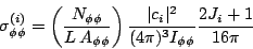
Now to convert the measured rate into a cross section we use the familiar luminosity and acceptance factors.
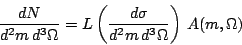 | (19) |
It is easy now to read off the
partial cross section for any wave i.
 | (20) |
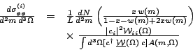
To get a total cross section for this wave, I integrate over masses and angles. The integral over masses converts to a sum over measured events as discussed above for Eq. 18.
 | (21) |
Here I have replaced the angular integral in the denominator with its
value as estimated from
Monte Carlo.
Last I do the angular integral, making use of the known normalization
properties of the
W
functions (see comments at the head of the wave4K source code.)
 | (22) |
This is the desired result. To obtain the errors arising from the
errors on x it might be easier just to calculate the values of
N![]()
![]() at the limits in x rather than doing a full propagation of errors.
The errors coming from the PWA coefficients are easy to calculate
analytically and can be added in quadrature to those coming from the
N
at the limits in x rather than doing a full propagation of errors.
The errors coming from the PWA coefficients are easy to calculate
analytically and can be added in quadrature to those coming from the
N![]()
![]() factor.
factor.
How do the results compare with the total cross section we published?
[RTJ] March 7, 2000
I am now convinced that the waves selected by Antimo give a satisfactory
description of the angular distributions of our
sample. Starting from the same input and same waves, we will find slightly
different amplitudes because we chose and weight the events differently in
the fit. However Table 7 says that our shapes are
in very good agreement, so if our parameters look different it is a measure
of the uniqueness of a fit to our data. By making adjustments to the shape
of the peak shape used to fit the Goldhaber plot, I was able to get rid of
the bias that had been skewing my
yields on the low side (see Table 4 and
Table 5). This change is already reflected in
Table 7.
In my way of doing the fit, I get out both the channel apportioning and
the pwa coefficients from the same fit. This allows me to go back and
recalculate the
cross section, this time using the fitted angular distribution in
calculating the acceptance instead of naively assuming phase space,
as we did in the PRD paper. So now I can go back and check that
assumption. The results are shown below in Table 8. The
PRD cross section values were interpolated from Table 1 in that paper,
without correcting for missing decay modes of the
.
| point no. |
momentum range (MeV) |
N (full fit) |
N (full fit) |
N (ch.likelhd.) |
N (ch.likelhd.) |
(�b) |
(�b) |
|---|---|---|---|---|---|---|---|
| 1 | 1180-1200 | 381 � 28 | 40 � 21 | 379 � 28 | 42 � 28 | 0.69 � 0.11 | 1.45 � 0.70 |
| 2 | 1220-1246 | 488 � 32 | 151 � 26 | 489 � 32 | 150 � 32 | 0.82 � 0.07 | 1.05 � 0.70 |
| 3 | 1260-1280 | 665 � 35 | 231 � 28 | 647 � 35 | 249 � 35 | 0.84 � 0.07 | 1.10 � 0.60 |
| 4 | 1300-1330 | 854 � 49 | 355 � 44 | 844 � 39 | 365 � 39 | 0.85 � 0.04 | 3.00 � 2.00 |
| 5 | 1345-1390 | 1011 � 36 | 583 � 30 | 1006 � 42 | 588 � 42 | 0.92 � 0.06 | 0.77 � 0.50 |
| 6 | 1390-1404 | 1251 � 46 | 596 � 38 | 1241 � 46 | 606 � 46 | 0.86 � 0.04 | 3.50 � 1.80 |
| 7 | 1405-1430 | 1738 � 43 | 931 � 32 | 1724 � 54 | 944 � 54 | 0.92 � 0.06 | 1.45 � 0.30 |
| 8 | 1435-1465 | 1358 � 46 | 885 � 41 | 1321 � 48 | 922 � 48 | 0.82 � 0.05 | 2.50 � 1.20 |
| 9 | 1465-1500 | 1214 � 34 | 981 � 30 | 1211 � 47 | 984 � 47 | 0.74 � 0.04 | 1.30 � 0.50 |
| 10 | 1505-1650 | 888 � 38 | 1111 � 40 | 860 � 42 | 1139 � 42 | 0.54 � 0.04 | 2.40 � 1.40 |
| 11 | 1700-1800 | 937 � 23 | 1591 � 34 | 926 � 46 | 1602 � 46 | 0.48 � 0.03 | 1.10 � 0.50 |
| 12 | 1900-2000 | 730 � 21 | 1643 � 37 | 739 � 42 | 1634 � 42 | 0.38 � 0.04 | 2.00 � 1.10 |
I was just looking over your phi phi pwa analysis web page/logbook, and had a quick question as to how I should interpret Table 8. In the last entry, 7 Mar 2000, I would expect the last two columns of the table to agree. The sigma(full fit) column, however, seems to always be around a sigma + a bit higher than the sigma(PRD) column, and the uncertainties are significantly higher. Am I making the correct comparison here? Is this the same comparison that I'm making if I compare the N(full fit) vs N(ch.likelhd.) where the numbers agree well?
The two columns sigma(PRD) and sigma(full fit) represent the same number, somehow. But we don't measure a total cross section in Jetset because of our limited acceptance. One way to get a total cross section is to make an assumption about the shape of the angular distribution, say just uniform phase-space. Then the yields just scale into a cross section with no inflation of errors. Another way is to get the shape from a fit to the angular distributions, and then integrate the shape to get the cross section. That way you get inflation of errors because the fit is unconstrained in regions where we have no data, but those regions contribute to the integral. So if the fit is underconstrained then you should see the errors blow up because of the uncertainty in how the shape extrapolates to regions of zero acceptance. When errors get larger than the estimated value and the estimator is positive definite by construction then there is a systematic bias on the high side of the best value. The conclusion from this is that phase-space underestimates our errors, a zillion-wave fit goes to the other extreme, and we are seeking a few-wave fit that is essentially as good but incorporates reasonable assumptions about the convergence of the expansion in angular momentum instead of an ad-hoc assumption of phase-space.
N is the yield after the total cross section has been multiplied by acceptance. Antimo's number N(ch.likelhd.) is just a fit of the Goldhaber plot. To get something to compare with him, I took the angular shape from the zillion-wave best fit for each point, froze the shape coefficients for the angular distributions and asked the fit to just tell me how much of the sample was phi,phi and how much background (parameterized as phase-space). The agreement shows that the channel apportioning gets the same answer independent of assumptions about angular distributions. This result had better be the case because the two factorize in the physical cross section. The agreement also shows that two different people using different tools on two different continents can do the same calculation and get the same answer.
Seeing Paul's reaction to Table 8, I think it would be more enlightening to look at similar quantities but where the 5-wave fit is being compared with the PRD values, where the total cross section should be better constrained. These results are shown below in Table 9.
| point no. |
momentum range (MeV) |
N (5-wave fit) |
N (5-wave fit) |
N (ch.likelhd.) |
N (ch.likelhd.) |
(�b) |
(�b) |
(�b) |
|---|---|---|---|---|---|---|---|---|
| 1 | 1180-1200 | 371 � 22 | 50 � 13 | 379 � 28 | 42 � 28 | 0.69 � 0.11 | 0.37 � 0.06 | 0.52 � 0.10 |
| 2 | 1220-1246 | 468 � 19 | 171 � 7 | 489 � 32 | 150 � 32 | 0.82 � 0.07 | 0.40 � 0.04 | 0.32 � 0.09 |
| 3 | 1260-1280 | 652 � 27 | 244 � 18 | 647 � 35 | 249 � 35 | 0.84 � 0.07 | 0.50 � 0.04 | 0.36 � 0.07 |
| 4 | 1300-1330 | 840 � 29 | 369 � 19 | 844 � 39 | 365 � 39 | 0.85 � 0.04 | 0.62 � 0.03 | 0.41 � 0.06 |
| 5 | 1345-1390 | 1005 � 31 | 589 � 23 | 1006 � 42 | 588 � 42 | 0.92 � 0.06 | 0.53 � 0.03 | 0.38 � 0.02 |
| 6 | 1390-1404 | 1245 � 32 | 602 � 20 | 1241 � 46 | 606 � 46 | 0.86 � 0.04 | 0.86 � 0.04 | 0.57 � 0.07 |
| 7 | 1405-1430 | 1732 � 38 | 936 � 25 | 1724 � 54 | 944 � 54 | 0.92 � 0.06 | 0.92 � 0.06 | 0.63 � 0.05 |
| 8 | 1435-1465 | 1333 � 33 | 910 � 26 | 1321 � 48 | 922 � 48 | 0.82 � 0.05 | 0.83 � 0.05 | 0.58 � 0.07 |
| 9 | 1465-1500 | 1206 � 29 | 989 � 25 | 1211 � 47 | 984 � 47 | 0.74 � 0.04 | 0.72 � 0.04 | 0.52 � 0.05 |
| 10 | 1505-1650 | 876 � 24 | 1123 � 28 | 860 � 42 | 1139 � 42 | 0.54 � 0.04 | 0.49 � 0.04 | 0.41 � 0.04 |
| 11 | 1700-1800 | 916 � 21 | 1612 � 33 | 926 � 46 | 1602 � 46 | 0.48 � 0.03 | 0.43 � 0.03 | 0.46 � 0.04 |
| 12 | 1900-2000 | 701 � 16 | 1672 � 35 | 739 � 42 | 1634 � 42 | 0.38 � 0.04 | 0.39 � 0.04 | 0.51 � 0.05 |
Data selection:
Certain data sets were excluded from the analysis that was used for our PRD paper because there were normalization problems. Notably, most of the 1994 data were excluded. These data are almost a third of our total statistics, and are included in the PWA because we considered that the normalization problem was only an issue of scale and not of the shape of the angular distributions. Also, the PWA data had a cut placed on the RICH to select 4K, whereas the RICH was not used in the PRD analysis.Acceptance:
The net acceptance depends on how the events are distributed in angles. The acceptance functions obtained from the fit are compared in Fig. 3. There are 15% jumps between points because of running under different trigger conditions, but generally the momentum-dependence is smooth. The total cross section comes from dividing the yield by acceptance, so increased acceptance results in a decreased cross section.
The last three columns in Table 9 require explanation.
The PRD
cross section is just what we published in 1998. The 5-wave fit
cross section in what comes back from the PWA fit for the total resonant
cross section when I put in the 5 waves recommended by Antimo. There
are three reasons for the differences between the PRD and
5-wave fit values.
The cross section column labeled flat in Table 9 was made to enable the separation of these two effects. To obtain the flat cross section values, I took the yields from my fit and corrected them with an acceptance calculated from the Monte Carlo I am using for the PWA, but assuming flat angular distributions. This takes out the acceptance effects, so any remaining discrepancy wiht the PRD value must come from item (1) above.
Several things emerge from looking at Fig. 3. The solid curve I obtained by digitizing the image from our PRD paper, Fig. 6a. I obtained the black points from the Monte Carlo used in this analysis without any weighting of angular distributions (i.e. events generated with uniform angular distributions). The departure of points 1-5 from the curve is interesting, and correspsonds to the discrepancy between the PRD and flat values for those points in Table 9. In drawing the curve the way we did in the PRD Fig. 6 I am guessing that we judged the acceptances for points 1-5 were too high. Is this correct Antimo?
In what follows, I am going to ignore any putative normalization corrections. We can discuss that later, as regards what we put into the paper for the sake of consistency with the former publication, but for the purposes of the PWA I am not going to fiddle. The red points in Fig. 3 follow a smooth curve, apart from wiggles that mimic those in the black dots. The question of resonances in our data set are independent of broad smooth deformations of the acceptance function, or at least had better be if we are to believe our conclusions. This is why we decided to include these data in the PWA in the first place. My conclusions are (1) that the change in the acceptance function due to angular distribution effects is real and large, but smooth as a function of beam energy, and (2) normalization questions affect the magnitude of the cross section at the low end of our energy range, but in examining the overall behavoior of the partial waves the acceptances from Monte Carlo will be taken at face value. Lets now go on and look at the results.
Do we have evidence for a resonance at 2.230?
[RTJ] March 24, 2000
The results of the PWA are given in Table 10.
The two different sets of solutions correspond to slightly different
parameterizations of the resonance
lineshape in the Goldhaber plot. Set B was obtained using a
double-Gaussian fit to the Monte Carlo
Goldhabber plot. The shape makes a good visual fit to the real
mass spectrum in the -band plot, but
gives a systematic bias towards low
yields when tested on known mixes of resonant and 4K Monte Carlo
as shown in Table 5. Set A was obtained by
tweaking the resonant lineshape in the Goldhaber plot until this bias
is removed. Set A tends to have longer tails to higher masses than
appears in the Monte Carlo mass plots, which explains why it finds more
in the data than set B. Visually, it is not possible to distinguish
the two lineshapes by examining the Goldhaber plot of the real. Hence
I consider the differences between sets A and B indicative of the
systematic errors implicit in the parameterization of the resonance
lineshape.
| wave no. |
Set A | Set B | ||
|---|---|---|---|---|
| cross section | relative phase | cross section | relative phase | |
| 11 | xs11a.eps | ph11a.eps | xs11b.eps | ph11b.eps |
| 12 | xs12a.eps | ph12a.eps | xs12b.eps | ph12b.eps |
| 13 | xs13a.eps | (reference wave) | xs13b.eps | (reference wave) |
| 15 | xs15a.eps | ph15a.eps | xs15b.eps | ph15b.eps |
| 16 | xs16a.eps | ph16a.eps | xs16b.eps | ph16b.eps |
| 20 | xs20a.eps | ph20a.eps | xs20b.eps | ph20b.eps |
| xsta.eps | xstb.eps | |||
The consistency between sets A and B is excellent and shows that we
are not sensitive to the details of the resonance lineshape. The
phases have been plotted with repeated data points every
2 so that the natural flow from point
to point is not interrupted by corssing through some arbitrary
principal value cut. What is not shown on the plot is that the
overall sign of the phases is not determined in the fit; there is an
overall sign ambiguity in the phase. That is unfortunate because we
cannot tell whether it is the 3++ wave or the 2++ waves that is
responsible for the resonant structure at 1.450 that is seen in the
relative phase between waves 15 and 13. I would argue from the
shapes of the partial cross section that the 2++ waves are responsible;
they all show some evidence of a peak around 1.450. Although no one
of them is overwhelming, the sum shows a clean enhancement there, and
the peak in the total cross ection is clearly coming from them.
Whatever you think of that argument, I think the answer to the
question, do we see a resonance at 2.230 with a narrow width decaying to
.
I think the answer is yes!
so that the natural flow from point
to point is not interrupted by corssing through some arbitrary
principal value cut. What is not shown on the plot is that the
overall sign of the phases is not determined in the fit; there is an
overall sign ambiguity in the phase. That is unfortunate because we
cannot tell whether it is the 3++ wave or the 2++ waves that is
responsible for the resonant structure at 1.450 that is seen in the
relative phase between waves 15 and 13. I would argue from the
shapes of the partial cross section that the 2++ waves are responsible;
they all show some evidence of a peak around 1.450. Although no one
of them is overwhelming, the sum shows a clean enhancement there, and
the peak in the total cross ection is clearly coming from them.
Whatever you think of that argument, I think the answer to the
question, do we see a resonance at 2.230 with a narrow width decaying to
.
I think the answer is yes!
So what's next? One thing anyone looking at these data is going to ask is, did you try extending wave 16 to the entire data set. If the resonance is 3++ you might see it in that wave as well. As it is, changing waves from 16 to 20 right in the vicinity of our peak might raise some questions. Antimo, did you every try a 6-wave hypothesis and use the same set of waves across the entire energy range?
I now try the 6-wave fit. First I have to find the new maximum likelihood
and check that including the extra wave makes a significant improvement to
the fit. Each time I redo the fit, I also make sure that the number of
from the
fit is reasonable. These numbers are not reported again; they are similar
to what was reported above in Table 8. For this
work I continue to work with Set A of Table 10 and
drop Set B. The following Table 11 shows the
improvement in the fit quality that comes from including the sixth wave
for each point.
| point no. |
momentum range (MeV) |
-ln(Lmax) (full fit) | -ln(L5) (5-wave fit) | -ln(L6) (6-wave fit) | 2 ln(Lmax/L5) | 2 ln(Lmax/L6) | correlation factor |
|---|---|---|---|---|---|---|---|
| 1 | 1180-1200 | 3239.9 | 3254.2 | 3251.5 | 28.6 | 23.3 | 0.969 |
| 2 | 1220-1246 | 4997.7 | 5018.2 | 5008.9 | 41.0 | 22.5 | 0.925 |
| 3 | 1260-1280 | 6851.0 | 6875.9 | 6873.2 | 49.8 | 44.4 | 0.970 |
| 4 | 1300-1330 | 8898.8 | 8930.4 | 8924.4 | 63.2 | 51.2 | 0.950 |
| 5 | 1345-1390 | 11842.4 | 11866.1 | 11863.8 | 47.4 | 42.8 | 0.958 |
| 6 | 1390-1404 | 12755.6 | 12774.0 | 12771.7 | 36.8 | 32.2 | 0.994 |
| 7 | 1405-1430 | 18297.1 | 18319.3 | 18316.0 | 44.4 | 37.8 | 0.992 |
| 8 | 1435-1465 | 15671.4 | 15690.4 | 15684.7 | 38.0 | 26.6 | 0.982 |
| 9 | 1465-1500 | 14897.9 | 14922.9 | 14920.4 | 50.0 | 45.0 | 0.997 |
| 10 | 1505-1650 | 13653.8 | 13684.4 | 13681.3 | 61.2 | 55.0 | 0.993 |
| 11 | 1700-1800 | 15948.2 | 15974.8 | 15968.2 | 53.2 | 40.0 | 0.992 |
| 12 | 1900-2000 | 14294.1 | 14318.6 | 14311.8 | 49.0 | 35.4 | 0.926 |
Antimo and I have had some discussion about how his fit results can be converted into partial cross sections. I have worked out the normalizations for both his approach and mine. Because it involves long formulas it was easier to write by hand and scan. The logbook entry is available here as a PDF file.
Useful links
[1] Antimo's logbook on partial wave analysis[2] Wave table listing the quantum numbers of the waves that are considered in the
 PWA.
PWA.
This page is maintained by Richard Jones.
Last modified