Difference between revisions of "Construction of a Tabletop Michelson Interferometer"
| Line 89: | Line 89: | ||
The last line is the actual search function. The search functions by finding the location with the smallest difference between the intensity(a(m,n)) and the fit function we apply to image. We use a gaussian distribution with user defined parameters as our fit. The code for this function is: | The last line is the actual search function. The search functions by finding the location with the smallest difference between the intensity(a(m,n)) and the fit function we apply to image. We use a gaussian distribution with user defined parameters as our fit. The code for this function is: | ||
| − | + | [[Image:Screenshot2.png|center|Matlab code used for image analysis]] | |
| − | |||
| − | |||
| − | |||
| − | |||
The parameters p(1) to p(6) are, in numerical order, (1) the amplitude of the function, (2) x location, (3)sigma x, (4) y location, (5) sigma y, and (6) an offset applied to eliminate background noise. The function takes user inputs as an initial guess, then loops the search process to find more accurate values for the parameters. Arbitrary values are chosen for p(1), p(3), p(5) and p(6) to begin, and are then readjusted based on the first output parameters. Typically, the closer these fit parameters are to the true parameters, the better the function is at defining p(2) an p(4). | The parameters p(1) to p(6) are, in numerical order, (1) the amplitude of the function, (2) x location, (3)sigma x, (4) y location, (5) sigma y, and (6) an offset applied to eliminate background noise. The function takes user inputs as an initial guess, then loops the search process to find more accurate values for the parameters. Arbitrary values are chosen for p(1), p(3), p(5) and p(6) to begin, and are then readjusted based on the first output parameters. Typically, the closer these fit parameters are to the true parameters, the better the function is at defining p(2) an p(4). | ||
By knowing the change in pixel location between photos, as well as th angular displacement, a value for pixel change per mrad in the x diection can be determined. This process is then repeated for the y direction. Once these two parameters are known, the video analysis can be used to find both frequency and amplitude. | By knowing the change in pixel location between photos, as well as th angular displacement, a value for pixel change per mrad in the x diection can be determined. This process is then repeated for the y direction. Once these two parameters are known, the video analysis can be used to find both frequency and amplitude. | ||
| − | {| | + | {| border="0" align="center" |
| − | |- | + | |- align="center" valign="top" |
| − | | [[Image: | + | | [[Image:false1.png|thumb|300px|]] |
| − | | | + | || [[Image:false2.png|thumb|300px|]] |
| + | |} | ||
| + | |||
| − | + | <br> | |
==Video analysis == | ==Video analysis == | ||
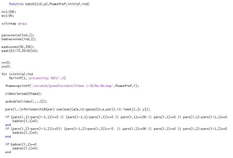
The same process used for the calibration images can be used to analyze the motion of the center of the lens flare over time. Because of the number of images involved in a video at 1200 fps, a batching process was developed to automate the process. First, a built in Linux program, ffmpeg, is used to separate the images from the video. Next, the automation script is applied to the folder containing the video stills. This script uses the same code as the image analysis, but loops the search process through a large group of images. | The same process used for the calibration images can be used to analyze the motion of the center of the lens flare over time. Because of the number of images involved in a video at 1200 fps, a batching process was developed to automate the process. First, a built in Linux program, ffmpeg, is used to separate the images from the video. Next, the automation script is applied to the folder containing the video stills. This script uses the same code as the image analysis, but loops the search process through a large group of images. | ||
Revision as of 00:08, 28 April 2010
The pupose of this page is to describe the work being done in the construction of a tabletop Michelson Interferometer. The purpose of this device in the scope of the project is two fold. First, the interferometer can be used to analyze the vibrational characteristics of a diamond wafer suspended from a wire frame. Second, the interferometer can be used to study the surface profile of a diamond wafer, allowing us to see the effects that different cutting and mounting techniques have on the final product. The main work does this semester has been on the vibrational aspects of the diamond mounting.
Construction
Parts List
The following is a lis of the parts used in the construction of the inerferometer, along with a brief descripton of the parts.
| Category | Item | Description |
| Beam Splitter | Beam Splitter Cube | (2cm)3, AR, 400-700nm |
| Kinematic Platform Mount | (2in)2 | |
| Prism Clamp | Large clamping arm | |
| Camera | Casio Ex-F1 | |
| Mirrors | Protected Silver Mirror | 25.4mm Dia., R≈98% |
| Mirror Holder | Standard 1" holder | |
| Kinematic Mirror Mount | Adjustable Kinematic mount for 1" holder | |
| Light Source | 532nm Green laser Module | 5mW, 5mm spot size, <1.4 mrad div. |
| Kinematic V-Mount | Small Mount with Attached Clamping Arm | |
| Beam Expander/Spatial Filter | Pinhole | 5μm, 10μm, 15μm, and 20μm pinholes |
| Pinhole Holder | 1/2" and 1" standard holder | |
| Small Plano-Convex Lens | f=50mm, 12.7mm Dia., AR coating | |
| Lens Holders | Holder for 1/2" and 1" optics lenses | |
| Large Plano-Convex Lens | f=150mm, 25.4mm Dia., AR coating | |
| Translation Stages | Small Linear Translation Stage | 1 dimension translation stage |
| 3-Axis Linear Translation Stage | 3 dimension translation stage | |
| Common Mechanics | Posts | 3/4" and 1" high posts, 1/2" Dia. |
| Post Holders | 1" high post holders | |
| Safety Equipment | Laser Safety Glasses | Green and Blue laser beam protection |
Images of Set-up
The following are images of the complete Michelson set-up
Estimating Camera Sensitivity
It is critical to understand the sensitivity of the camera to light from the interferometer, given the high intended image acquisition speed. The camera purchased for this setup, Casio EX-F1, has a movie frame rate capability of 1200 Hz. The following information allows an order of magnitude estimate of the sensitivity. (The camera uses a CMOS sensor. Note that lx=lm·m2)
- a sample CMOS chip, Micron's MT9P401, has sensitivity of 1.4 V/lx·s and supply voltage of 2.8 V yielding 2 lx·s of light energy to saturation.
- Light intensity conversion - 320 lm/W given:
- a 100 W incandescent light bulb is measured to have the perceived intensity of about 1600 lm
- a rough figure of efficiency for a 100 W is 5%
Using these conversions, the sensor pixels saturate at 6.3×10⁻³ W·m2·s. At 1200 Hz acquisition rate, assuming 100% duty cycle, the saturation figure is 5.2×10⁻⁶ W·m.
Now, let us assume that only about 5% of 1 mW laser light reaches the sensor due to cleanup in the beam expander and the light transmitted through the diamond. If the light is expanded to a 2 cm diameter beam, the beam at the sensor is rated at 1.6×10⁻⁸ W·m2
The two order of magnitude shortfall means that very little of the dynamic range of the sensor will be used, leading to a low signal to noise ratio. For this reason, a 5mW laser was chosen over a 1mW.
Camera Calibration
Analysis of videos taken of the vibration of the diamond wafer can lead to information about both the frequency and the amplitude of vibration. To perform simultaneous measurements of both parameters, a precise camera calibration was necessary.
Calibration Set-Up
The following is an image of the device used for the camera calibration:
IMAGE OF CALIBRATION DEVICE
This calibration device was used to determine the change in pixel location of the center of the lens flares based on angular displacement. To do this, the camera was mounted horizontally on a 1.40m long bar. The camera end was free to rotate about a pivot located at the opposite end of the rod, above which a mirror was mounted. A linear micro-adjustment translation stage was placed below the camera end.
Image Analysis
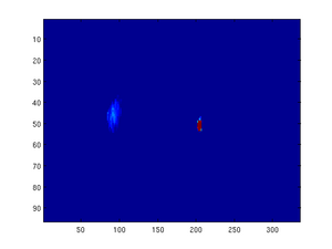
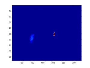
To find the location of the center of the flair on each image, several lines of code were implemented:
- The first line imports the image, in this case IMAG0001.jpg, converts it to a matrix, and separates the green channel. Next, this matrix is imaged in false color in terms of intensity from blue(low) to red(hgh).
The last line is the actual search function. The search functions by finding the location with the smallest difference between the intensity(a(m,n)) and the fit function we apply to image. We use a gaussian distribution with user defined parameters as our fit. The code for this function is:
The parameters p(1) to p(6) are, in numerical order, (1) the amplitude of the function, (2) x location, (3)sigma x, (4) y location, (5) sigma y, and (6) an offset applied to eliminate background noise. The function takes user inputs as an initial guess, then loops the search process to find more accurate values for the parameters. Arbitrary values are chosen for p(1), p(3), p(5) and p(6) to begin, and are then readjusted based on the first output parameters. Typically, the closer these fit parameters are to the true parameters, the better the function is at defining p(2) an p(4). By knowing the change in pixel location between photos, as well as th angular displacement, a value for pixel change per mrad in the x diection can be determined. This process is then repeated for the y direction. Once these two parameters are known, the video analysis can be used to find both frequency and amplitude.
Video analysis
The same process used for the calibration images can be used to analyze the motion of the center of the lens flare over time. Because of the number of images involved in a video at 1200 fps, a batching process was developed to automate the process. First, a built in Linux program, ffmpeg, is used to separate the images from the video. Next, the automation script is applied to the folder containing the video stills. This script uses the same code as the image analysis, but loops the search process through a large group of images.


