Next: About this document ...
Technical Note
radphi-2001-402
Energy calibration of the Radphi Lead Glass Detector
Richard Jones
University of Connecticut, Storrs CT
April 1, 2001
Abstract:
The Radphi experiment requires an energy calibration procedure
for the lead glass calorimeter. In the absence of an available source of
mono-energetic electrons or photons, the gains of the individual blocks
as well as the overall energy scale must be determined based only on
characteristic peaks that appear in the invariant mass spectra from
reconstructed showers. A procedure is described that reliably extracts
absolute gain coefficients for all 620 instrumented blocks from a sample
containing of order

events. These events are a subset of the
standard physics trigger, allowing redundant checks and time-dependent
calibration to be carried out after the data are already collected.
The LGD calibration procedure is based upon the fact that when the
positions and energies of individual showers in the calorimeter are
combined to form invariant an mass, the mass spectrum exhibits prominent
peaks corresponding to known mesons decaying into  final
states, eg.
final
states, eg.  ,
,  ,
,  ,
,  . These peaks are visible
in the reconstructed spectra even before the gain calibration has been
carried out, with individual tubes varying in gain by a factor of 2 or
more. The gains were set during the experimental run by adjusting the
high voltage on individual tubes until their responses to an injected
light pulse from the calibration laser were approximately equalized.
The pulser equalization procedure was repeated periodically throughout
the run to take into account changes in the response of individual blocks
arising from radiation damage and other sources of long-term drift during
the experiment. Inhomogeneities in the light distribution led to
physical gains on particular channels that differed by more than a
factor of two from the mean, with a 25% r.m.s. deviation. The goal
of the offline calibration is to measure these gain factors using
experimental data, so that they can be used in turn to correct the data
during reconstruction.
. These peaks are visible
in the reconstructed spectra even before the gain calibration has been
carried out, with individual tubes varying in gain by a factor of 2 or
more. The gains were set during the experimental run by adjusting the
high voltage on individual tubes until their responses to an injected
light pulse from the calibration laser were approximately equalized.
The pulser equalization procedure was repeated periodically throughout
the run to take into account changes in the response of individual blocks
arising from radiation damage and other sources of long-term drift during
the experiment. Inhomogeneities in the light distribution led to
physical gains on particular channels that differed by more than a
factor of two from the mean, with a 25% r.m.s. deviation. The goal
of the offline calibration is to measure these gain factors using
experimental data, so that they can be used in turn to correct the data
during reconstruction.
A calibration procedure based solely upon the reconstructed masses
of known mesons is apparently problematic because it seeks to exploit
one constraint (the known mass of the meson) to estimate multiple
parameters (gain correction factors for every channel that contributes
energy to the event). When many events containing a contribution from
a given block are superimposed, however, the dependence of the average
reconstructed mass on the gains of other blocks tends to wash out,
leaving a bias that comes from the gain of the block itself. Removing
this bias by applying a gain correction to this channel leads to a
narrower peak in the mass plot. This is accomplished quantitatively
by adjusting individual gain factors to optimize a single global
function of the data, shown in Eq. 1.
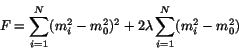 |
(1) |
where  is the number of events in the calibration data sample and
  denotes a single event in that sample. The masses
  and
and  are
the physical mass of the meson being used for the calibration and the
reconstructed mass in the LGD for event . The first term in
are
the physical mass of the meson being used for the calibration and the
reconstructed mass in the LGD for event . The first term in  measures the width of the reconstructed mass peak, while the second
term is introduced with the Lagrange multiplier
measures the width of the reconstructed mass peak, while the second
term is introduced with the Lagrange multiplier  to embody the
constraint
to embody the
constraint
 .
.
For the purposes of Radphi,
the most convenient meson for calibration turned out to be the
which appears as the dominant structure in the  invariant mass
plot for 2-cluster events. All events that were reconstructed with exactly
two clusters and whose invariant mass lay within
invariant mass
plot for 2-cluster events. All events that were reconstructed with exactly
two clusters and whose invariant mass lay within  % of the center
of the peak were candidates for the calibration sample. The
invariant mass is given by Eq. 2.
% of the center
of the peak were candidates for the calibration sample. The
invariant mass is given by Eq. 2.
 |
(2) |
where  ,
,  are the reconstructed energies of the two showers
and
are the reconstructed energies of the two showers
and  is the angle between the centers of the two showers as
viewed from the target.
is the angle between the centers of the two showers as
viewed from the target.
The reconstructed energy  is approximately
equal to the observed energy
is approximately
equal to the observed energy  in shower
  , but contains additional
nonlinear corrections to account for angle-dependent attenuation and output
coupling effects.
, but contains additional
nonlinear corrections to account for angle-dependent attenuation and output
coupling effects.
 |
(3) |
where  labels an individual block contributing to shower .
The nonlinearity correction factor
labels an individual block contributing to shower .
The nonlinearity correction factor  is weakly dependent on
the observed shower energy but not on the block energies
is weakly dependent on
the observed shower energy but not on the block energies
 individually. A calibration step consists of introducing a
small channel-dependent gain correction factor
individually. A calibration step consists of introducing a
small channel-dependent gain correction factor  such that
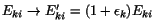 , where the prime
is used to denote the corresponding quantity after the gain correction
is applied.
, where the prime
is used to denote the corresponding quantity after the gain correction
is applied.
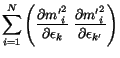
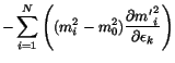
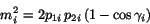
Minimizing in Eq. 1 directly with respect to the
variables is made difficult by the nonlinear dependence
of on the block energies that appears in the factor in
Eq. 3 and also in . Progress can be made by observing
that small shifts in the gain of a single channel will have little effect
on the nonlinear correction factors or the shower centroids, but will
rescale the of its shower as shown in Eq. 4.
 |
(4) |
 |
(5) |
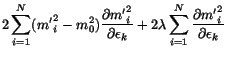
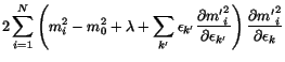
These approximations lead to a linear equation which is satisfied at the
minimum of the penalty function .
The solution is given by
![\begin{displaymath}
\epsilon_k = [C^{-1}]_{kk'} (D - \lambda L)_{k'}
\end{displaymath}](img37.png) |
(7) |
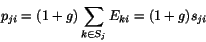
where
and the value of is fixed by the condition that the centroid
of the reconstructed mass peak must lie at the physical mass.
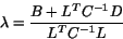 |
(8) |
where  is the mass bias
 . Starting
off with a nominal gain factor of unity for all channels, gain corrections
are calculated using Eq. 7 and applied iteratively until
the procedure converges to
. Starting
off with a nominal gain factor of unity for all channels, gain corrections
are calculated using Eq. 7 and applied iteratively until
the procedure converges to
 for all .
In practice, it was found that special care must be taken in the way
that the matrix
for all .
In practice, it was found that special care must be taken in the way
that the matrix  is inverted. is a square symmetric matrix with
620 rows and columns whose elements are determined statistically by
sampling a finite sample of calibration events. Even for very
large samples there are instabilities that appear when taking the
inverse
is inverted. is a square symmetric matrix with
620 rows and columns whose elements are determined statistically by
sampling a finite sample of calibration events. Even for very
large samples there are instabilities that appear when taking the
inverse  which demand careful treatment. The nature of these
instabilities can be best understood by expressing in terms of
its spectral decomposition Eq. 9.
which demand careful treatment. The nature of these
instabilities can be best understood by expressing in terms of
its spectral decomposition Eq. 9.
![\begin{displaymath}[C^{-1}]_{kk'} = \sum_{\alpha} \frac{1}{c(\alpha)}
e_k(\alpha) e_{k'}(\alpha)
\end{displaymath}](img50.png) |
(9) |
where  are the eigenvalues and
  the
corresponding orthonormalized
eigenvectors of . Of the 620 eigenvalues of , there are generally
a few whose values are very small and statistically consistent with
zero. These terms tend to dominate the behavior of if it is
calculated using exact methods. A better approach instead is to truncate
Eq. 9 and include only eigenvectors in the sum whose eigenvalues
are adequately determined by the data. This truncation implicitly
recognizes that there are some linear combinations of the gains which
cannot be determined from the given data sample, and simply leaves them
unchanged from the initial conditions. It is not the same as fixing any
subset of the values to zero on a given step, which does not
occur when this method is followed. Empirically it was found that good
convergence was obtained after 8-10 iterations of the above procedure.
the
corresponding orthonormalized
eigenvectors of . Of the 620 eigenvalues of , there are generally
a few whose values are very small and statistically consistent with
zero. These terms tend to dominate the behavior of if it is
calculated using exact methods. A better approach instead is to truncate
Eq. 9 and include only eigenvectors in the sum whose eigenvalues
are adequately determined by the data. This truncation implicitly
recognizes that there are some linear combinations of the gains which
cannot be determined from the given data sample, and simply leaves them
unchanged from the initial conditions. It is not the same as fixing any
subset of the values to zero on a given step, which does not
occur when this method is followed. Empirically it was found that good
convergence was obtained after 8-10 iterations of the above procedure.
Next: About this document ...
Richard T. Jones
2004-04-30