Predictions

In this section I convert the Monte Carlo numbers into predictions for the rates in each level of the Radphi trigger. The calculation relies on the model for the Radphi trigger presented in a previous note [1]. The parameters of the model were carefully calibrated using measurements taken during 1998 parasitic running. These parameters are carried over without change for this study, except that the rate in the UPV has been lowered by a factor of 5 to account for its having been moved upstream of its former position. The basic rate for the BSD triple-coincidence is taken to be the same as was measured for the RPD coincidence in 1998. Accidental coincidences between BSD layers are incorporated in addition to the basic ``pixel'' rate. The results are shown in Table 3. The BSD threshold was set at the maximum of the minimum-ionizing peak to obtain the reduction from the inclusive rates shown in Table 1. The difference between actual and scaler rates have to do with the dead time correction associated with each signal. For detector or signals, the scaler rates are suppressed relative to the actual rates because the signals have a finite duration and the scaler only counts lead edges. For the level 1 trigger rate the scaler does not reflect the dead time imposed by the BUSY signal, whereas the actual rate does.

Table 3: The rates expected in all levels of the Radphi trigger from the front end to the tape, based upon measurements taken during 1998 running and this study. All rates are normalized to running with 50nA electron beam at 5.5GeV energy and a $5\cdot 10^{-4}$ radiation length radiator.

signal		actual		scaler
tagger or		48		MHz		30		MHz
CPV or		67		MHz		34		MHz
UPV or		750		KHz		740		KHz
BSD layer 1		3.9		MHz		3.8		MHz
BSD layer 2		2.0		MHz		2.0		MHz
BSD layer 3		1.2		MHz		1.2		MHz
BSD layer $1\cdot 2$		1.1		MHz		1.1		MHz
BSD layer $1\cdot 3$		590		KHz		590		KHz
BSD layer $2\cdot 3$		590		KHz		590		KHz
BSD $1\cdot 2\cdot 3$		440		KHz		440		KHz
$BSD \cdot \overline{UPV}$		390		KHz		390		KHz
level 1 trigger		73		KHz		150		KHz
level 2 trigger		8.3		KHz		8.3		KHz
level 3 trigger		1.0		KHz		1.0		KHz
level 2 dead time		1.2		$\mu$s/event		(9%)
level 3 dead time		14		$\mu$s/event		(12%)
daq dead time		300		$\mu$s/event		(30%)
total live time		50%		@ 1KHz

Figure 10: Predicted rate of writing good triggers to tape vs electron beam current for a $5\cdot 10^{-4}$ radiation length radiator.

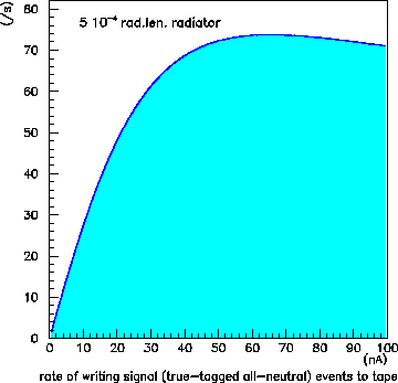Running an experiment with 50% live time is not unreasonable, as can be seen from Fig. 10. This plot shows the rate at which signal is being written to tape. What is meant by signal can be illustrated by a simple analysis in which all events with charged tracks (besides the recoil proton) are removed and then the time between the trigger and the tagger is plotted for the remaining events. In this plot appears a peak reflecting prompt coincidences surrounded by accidental background. The statistics in the coincidence peak, after accidentals are subtracted, is what is meant by signal. Of course the separation of signal from non-signal is only possible on a statistical basis. But in a tagged photon beam it is this quantity shown in Fig. 10 that is the figure of merit as far as statistics are concerned. This graph shows that the experiment profits from increased beam current all the way to 50nA, where it saturates.