


Next: Bibliography
Up: lgd_res
Previous: lgd_res
The energy and spatial resolution in the LGD are measured
using 2-shower invariant mass distributions from
 and
and
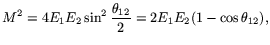
 decays, exploring the formula
for the square of the invariant mass
decays, exploring the formula
for the square of the invariant mass
 |
(1) |
where  and
and  represent photon energies, while
 is their angular separation. The variance
of the squared invariant mass in terms of the variances of energy and
shower position in the LGD is given by
is their angular separation. The variance
of the squared invariant mass in terms of the variances of energy and
shower position in the LGD is given by
![$\displaystyle V(M^2) = \sum_{i=1}^{2} \left[ \
\left(\frac{\partial M^2}{\part...
...rtial x_i}\right)\left(\frac{\partial M^2}{\partial y_i}\right) V_{XY} \right],$](img12.png) |
(2) |
where index  counts photons.
The expression for the energy resolution
counts photons.
The expression for the energy resolution
 is
given by Eq. 2 (NIM:
is
given by Eq. 2 (NIM:
 )
where parameters
)
where parameters  and
and  have to be determined.
Spatial variances are taken to be
have to be determined.
Spatial variances are taken to be
where  depends on the size of the LGD block,
and
depends on the size of the LGD block,
and  is radiation length [1].
For this LGD
is radiation length [1].
For this LGD  mm
mm GeV
GeV
 , and
, and
 mm [2].
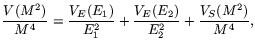
Finding energy derivatives from Eq. 2 is straight forward while all
spatial derivatives can be expressed in terms of measured photon momenta
[3]. Taking all this into account,
Eq. (2) can be simplified as
mm [2].
Finding energy derivatives from Eq. 2 is straight forward while all
spatial derivatives can be expressed in terms of measured photon momenta
[3]. Taking all this into account,
Eq. (2) can be simplified as
 |
(4) |
where spatial derivatives and variances are grouped into the term  .
From events with two reconstructed showers the
.
From events with two reconstructed showers the  sample was selected
by limiting invariant mass to
sample was selected
by limiting invariant mass to 
 and the
  sample was
obtained by selecting pairs with shower separation
sample was
obtained by selecting pairs with shower separation

 .
The mass resolution was measured by forming the invariant mass
distributions for a set of well-defined shower energies
.
The mass resolution was measured by forming the invariant mass
distributions for a set of well-defined shower energies
 , with
 for the and
 for
the sample.
The and peaks from these distributions were
fitted with a Gaussian over a polynomial background.
From the Gaussian fit the value
for
the sample.
The and peaks from these distributions were
fitted with a Gaussian over a polynomial background.
From the Gaussian fit the value
 has been
calculated. The errors are predominantly systematic, governed by the
choice of background function, and estimated to be
has been
calculated. The errors are predominantly systematic, governed by the
choice of background function, and estimated to be  and
and  for the and data respectively.
Examining the distributions from and decays
it was seen that spatial part in the mass resolution
is at level, while it gives significant
for the and data respectively.
Examining the distributions from and decays
it was seen that spatial part in the mass resolution
is at level, while it gives significant  contribution to
the mass width [3].
Consequently, in the first approximation the spatial
contribution to the mass resolution has been neglected.
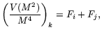
Following Eq. (4) the set of
contribution to
the mass width [3].
Consequently, in the first approximation the spatial
contribution to the mass resolution has been neglected.
Following Eq. (4) the set of  equations
 |
(5) |
was formed, where indexes  map different photon energies being used.
The least-square solution for the
map different photon energies being used.
The least-square solution for the  values,
 ,
was found without assuming the functional form of
,
was found without assuming the functional form of  .
This model-independent solution is free of any restrictions on the
.
This model-independent solution is free of any restrictions on the
 values except that
  for
for  . The corresponding
 from the free solution is plotted
in Fig. 1. These points agree very well
with the standard expression for the energy resolution (Eq. 2),
with
from the free solution is plotted
in Fig. 1. These points agree very well
with the standard expression for the energy resolution (Eq. 2),
with  and
and  GeV
.
In the next step, the spatial corrections to the mass resolution
has been included by recording the mean of the
GeV
.
In the next step, the spatial corrections to the mass resolution
has been included by recording the mean of the
 distributions for each (
 ) choice, for both the and
samples. The expression for the variance function
(Eq. (4)) was modified, using the standard expression
for the energy resolution,
) choice, for both the and
samples. The expression for the variance function
(Eq. (4)) was modified, using the standard expression
for the energy resolution,
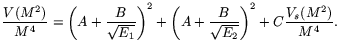 |
(6) |
In addition to the parameters and , parameter
 that scales the spatial resolution contribution has been introduced.
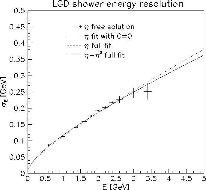
Within this simple model the data fit with set to zero is shown as
solid line in Fig. 1, while the fit parameters are shown in the
first row of Table 1. The data fit when was let to
vary is represented by the dashed line in Fig. 1 and the
second row in Table 1. The fit confirms that the mass
resolution is not very sensitive to spatial corrections.
In the next step all measured points from the and samples
were fitted together. The fit is shown as the dotted line in Fig. 1,
and the resulting parameters are shown in the last row of Table 1.
Both the and mass distributions are described well
with this single set of parameters.
The scale parameter can be viewed as a correction to
the nominal value of mmGeV
for the LGD,
since the energy-dependent term in the spatial errors is dominant at
small and moderate angles
that scales the spatial resolution contribution has been introduced.
Within this simple model the data fit with set to zero is shown as
solid line in Fig. 1, while the fit parameters are shown in the
first row of Table 1. The data fit when was let to
vary is represented by the dashed line in Fig. 1 and the
second row in Table 1. The fit confirms that the mass
resolution is not very sensitive to spatial corrections.
In the next step all measured points from the and samples
were fitted together. The fit is shown as the dotted line in Fig. 1,
and the resulting parameters are shown in the last row of Table 1.
Both the and mass distributions are described well
with this single set of parameters.
The scale parameter can be viewed as a correction to
the nominal value of mmGeV
for the LGD,
since the energy-dependent term in the spatial errors is dominant at
small and moderate angles
 , while the angular part
in Eq. (3) becomes important only at large angles
, while the angular part
in Eq. (3) becomes important only at large angles
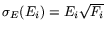
 . According to the fit results the energy resolution function is

,
while the shower position uncertainty can be expressed as

,

,
where ( ) are the polar coordinates of the shower in the face of
the LGD. All lengths in these relations are in mm and all energies in GeV.
) are the polar coordinates of the shower in the face of
the LGD. All lengths in these relations are in mm and all energies in GeV.
Table 1:
The parameter values from different fits to the and
mass resolutions, obtained using Eq. (6). The corresponding
fits are shown in Fig. 1
| Fit |
|
![$ \left[GeV^{-1/2}\right]$](img65.png) |
|
 |
( ) ) |
 |
 |
0 |
1.05 |
| (full) |
 |
 |
 |
1.04 |
 (full) (full) |
 |
 |
 |
1.50 |
Figure 1:
Energy resolution of showers in the LGD obtained from analysis of the
 sample. Points represent the free solution to the
mass resolution measurements when the contribution from the spatial
resolution has been neglected. The solid line represents the fit to the
data with the standard energy resolution model (Eq. (6)with ).
The dashed line represents the fit to the data when the spatial
contribution is taken into account by Eq. (6). The dotted line
corresponds to the simultaneous fit to the and data with the
same function (Eq. (6)). Corresponding fit parameters and
are shown in Table 1.
sample. Points represent the free solution to the
mass resolution measurements when the contribution from the spatial
resolution has been neglected. The solid line represents the fit to the
data with the standard energy resolution model (Eq. (6)with ).
The dashed line represents the fit to the data when the spatial
contribution is taken into account by Eq. (6). The dotted line
corresponds to the simultaneous fit to the and data with the
same function (Eq. (6)). Corresponding fit parameters and
are shown in Table 1.
 |
Next: Bibliography
Up: lgd_res
Previous: lgd_res
Mihajlo Kornicer
2003-12-11