Calculating the move
Calculating Position of Each Bundle Support Mounting Rod
An Excel spreadsheet has been created to calculate the location of the bundle supports' mounting rods with respect to the focal plane coordinate system. This spreadsheet also calculates the length of the parallel railing end supports which need to be fabricated anew for each unique TAGM location on the focal plane. One last, but very important thing that the spreadsheet calculates is the shim size needed, during TAGM realignment, in order to achieve the proper tow angle between bundle supports during mounting. In addition to the spreadsheet, an AutoCAD drawing used to design the three parallel rail components needed for each unique tagging energy spectrum starting position of the TAGM and a drawing for the current setup (β = 12.5o to 11.06o). These files are in US standard units (inches) and to scale with a tolerance of ± 0.001 inch.
A summary of the spreadsheet calculations is a follows:

- Select a starting energy for the photon tagging array (highest γ energy to tag)
- Using hodoscope energy bin bounds interpolate the crossing angle with respect to the focal plane (β1) of an electron associated the highest energy to be tagged (Eγo)
- Interpolate the location on the XFP axis at which this electron crosses (X1)
- These electrons will pass through the center of the first column of SciFi fibers
- Using β1 calculate the X-displacement along the focal plane (Δx) from the center of the first fiber column to the center of the sixth fiber column of the first bundle support
- Add Δx and X1 to get X6, then interpolate the value of β6
- Using the average value of β1 and β6 (βavg.), recalculate the XFP displacement (Δx) from the center of the first to sixth fiber column (X6)
- Repeat the above two steps until the bundle support angle β (e.g. average between β1 & β6) does not change appreciably
Now we know the focal plane crossing locations for the center of the first and sixth SciFi columns in our first bundle, as depicted in Figure 1 by the endpoints of Δx. Additionally, we know the β angle of the first bundle (noted as βavg above), which gives us the optimal alignment for each fiber in the bundle to their respective electron's path. The β angles for the first and sixth columns will be off by the same magnitude, but with opposite signs.

The 5x6 fiber bundle supports were designed with two 5x3 bundle halves offset such that the center of the front face of the middle column in each bundle half would sit on the magnetic focal plane for a β angle of 12.0o. This angle was selected as a compromise that would allow coverage through the photon energy range of 10 - 5.6 GeV.
As a side note - If required and finances permit, the 17 bundle supports can be easily redesigned for a different β angle. This redesign would take less than an hour of CAD work, with a manufacturing turn-around time in as little as two days. Costs are estimated to be around $5k. A CAD drawing of a new bundle support design, with the current forward and rear bundle half stagger, already exists. This new design incorporates updated locations of the threaded holes for mounting the clamps that keep the bundle straps in place; thereby, permitting a slightly larger range of coverage on the focal plane and a more secure way to hold the fiber straps. The best time to replace/modify the bundle supports, if so desired, would be during fiber replacement. This way the new fibers can be mounted to the new bundle support outside the tagger hall, before ever making it to JLab. A conservative time estimate for changing the TAGM fiber configuration would be approximately two days (16 hours).
Each bundle has a "pivot point" that when placed on the focal plane, provides the optimal y-displacement from the focal plane for each fiber column in that bundle without encroaching too close to the tagger magnet window. If the bundle β angle ≠ 12o, then the 1st & 6th, 2nd & 5th, and 3rd & 4th fiber column pairs will have the same magnitude offset as one another from the focal plane in Y, but with opposite signs, see Figure 2. This is all provided that when the bundle support is mounted on the parallel railing system the tagger magnet's focal plane passes through the midpoint between the front and rear bundle halves (the so called pivot point).

As shown in Figure 3 by the red and green lines, if β ≠ 12o then the front face of the first column of SciFi no longer sits on the focal plane. This offset must be accounted for. The Excel spreadsheet starts by finding the optimal first bundle support crossing angle (βavg) and places the front center of the first column of SciFi on the XFP location corresponding to Eγo. Depending on β's departure from 12o the pivot point will be displaced from the focal plane. The spreadsheet calculates the (Δx, Δy) needed to return the pivot point to the focal plane and keep the first fiber column's longitudinal axis on the Eγo electron's path. The spreadsheet's title for this is "Pivot Point Move" and the description is detailed below.
NOTE: βavg is used to determine this displacement. While the Eγo electron's β angle differs slightly βavg and would keep the column's centerline on the proper electron path, this discrepancy is so small that it does not come close to the TAGM machining parts' tolerance. Additionally, the sixth column's β angle has the same magnitude difference from the bundle support's β, but with a different sign. For these reasons βavg was used.
- Pivot Point Move for β ≠ 12 deg.
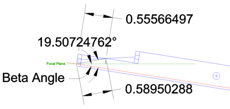
Figure 4: Dimensions of the pivot point to the front center of the first column of fibers. The three 2 mm2 boxes at the end of each 5x3 bundle half are only included to represent the width of a fiber column and have no meaning in length in the longitudinal axis direction.
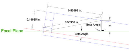
Figure 5: Dimensions of the pivot point to the front center of the first column of fibers. The three 2 mm2 boxes at the 5x3 bundle half are only included to represent the width of a fiber column and have no meaning in length in the longitudinal axis direction.
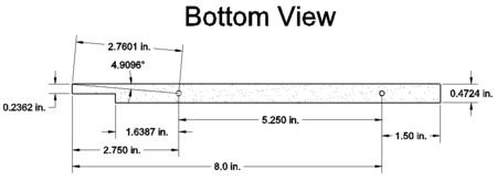
Figure 6: Dimensions of the bundle support as viewed from below. This view shows the location of the bundle support mounting rods at 2.75 in. and 8 in. from the front of the bundle support.


- Calculate the YFP displacement required to place the focal plane back on the bundle support's pivot point, Figure 5
- The angle made by the first fiber column's longitudinal axis and a line from (X1, 0)FP to the pivot point is 19.5072o, see Figure 4
- Use the difference between βavg and 19.5072o
- The distance of the center of the first fiber column's front face to the bundle support's pivot point (in the (x, y)FP plane) is 0.5895 inches
- Note that if β > ~19.5o (e.g. > 10.86 GeV photons being tagged), then the pivot point will be below the focal plane; therefore, Δy will be positive (bundle shifts towards the magnet, positive YFP direction)
- Utilizing the y-displacement value found above and the tangent of βavg, calculate the associated x-displacement along the focal plane to keep column #1 aligned to the electrons associated with Eγo


- Next determine the locations of the bundle support mounting rods in focal plane coordinates
- Figure 6 shows the required dimensions for these calculations
- For x locations, include x1 (for Eγo electrons) in addition to the rods' displacement from the front center of the first fiber column
- For y locations, we assume y1 (for Eγo electrons) lies on the focal plane y-axis
- The Excel spreadsheet provides calculations for the corners of the upstream bundle halves for each bundle support. As shown in Figure 9 below, it is easiest to determine the forward rod location from the upstream bundle half corner closest to the magnet.
- The rear support rod is 5.25 inches, see Figure 6, from the forward support rod along the bundle support's longitudinal axis.

Fitting the Position of Each Bundle Support Mounting Rod to a Straight Line
At this point the exact location for each bundle support rod is known. These locations place the scintillating fibers of each bundle support at their optimal location. Unfortunately these locations deviate slightly from a straight line. To correct this deviation and find a compromise the their location that's within the TAGM required tolerance, we must use ROOT and fit a first order polynomial to the calculated locations. A template C++ file has been written for this purpose. Once the arrays used for the rods' x and y locations are updated for the desired tagging energy spectrum, then the macro can be run or the code can be copy & pasted directly into ROOT's command line. The generated histograms, for the forward and rear rods, can then be fitted to a first order polynomial (pol1) using the Fitting Tool. Several fit equations are already recorded in a fit function repository file. The fits are then utilized back in the Excel file to determine the "Y-Fit" location for each rod X location. This way the parallel rails can be orientated based on these numbers and the three rail components required for the TAGM move can be designed.
- Fitting the calculations to real life
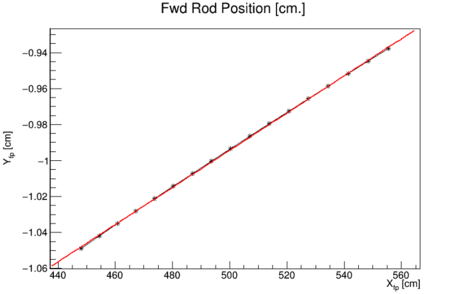
Figure 10: Histogram of the bundle supports' forward rod position (*) in focal plane coordinates. The red line is a first order polynomial fit (pol1) using the ROOT fitter.
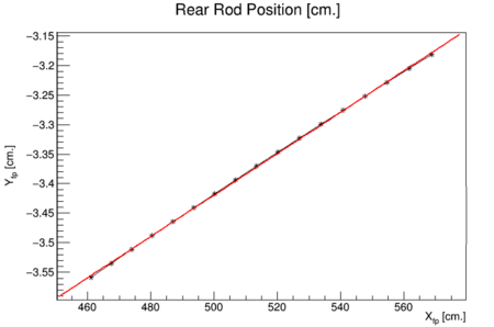
Figure 11: Histogram of the bundle supports' rear rod position (*) in focal plane coordinates. The red line is a first order polynomial fit (pol1) using the ROOT fitter.


- Copy and paste the locations for the bundle support rods into the the fitting file and run in ROOT.
- Fit the histograms to a straight line (pol1) and input the resulting fit equations into both fit function repository file and the Excel file for calculating bundle support locations
- The Excel file will provide the "Fit-Y" locations that are used in the CAD drawing to design the three unique parallel rail pieces that are needed for each TAGM move.
- Using [http: Beta_Manipulation2.dwg], rotate each bundle support by its β angle then locate the forward rod at the fit position determined by the previous step.
- With all bundle supports in the fit determined location (forward rod), draw a straight line through the center of the forward rods and through the best fit of the rear rods.
- Using these two straight lines realign the parallel rails.
- The Excel file also contains a distance from the parallel rail upstream tapped hole to where the first bundle should start, so as to allow for screw heads to fit.
- Finally use CAD to design the parallel rail support components needed for the move. See below, Figure 12 - 18, for the 6 GeV starting point drawings.


