Difference between revisions of "Hybrid Photodiode"
Senderovich (talk | contribs) m |
Senderovich (talk | contribs) m (→Results) |
||
| (7 intermediate revisions by the same user not shown) | |||
| Line 73: | Line 73: | ||
\left( \begin{matrix} n\\k \end{matrix} \right) | \left( \begin{matrix} n\\k \end{matrix} \right) | ||
(1-\alpha-\beta)^{m-n} \alpha^{n-k} \beta^{k} | (1-\alpha-\beta)^{m-n} \alpha^{n-k} \beta^{k} | ||
| − | \ G\left( (m-n) + (n-k)p + kr,\ (m-n)\sigma_1^2 + (n-k)\sigma_2^2 + k\sigma_3^2 \right) | + | \ G\left( (m-n) + (n-k)p + kr,\ \sigma_0^2 + (m-n)\sigma_1^2 + (n-k)\sigma_2^2 + k\sigma_3^2 \right) |
</math> | </math> | ||
| Line 87: | Line 87: | ||
* Pedestal position: -3.6606 × 10<sup>-3</sup> V; | * Pedestal position: -3.6606 × 10<sup>-3</sup> V; | ||
| − | The parameters relating to the shape of the primary and secondary electron distributions, as well as an additional Gaussian noise factor were allowed to vary. | + | The parameters relating to the shape of the primary and secondary electron distributions, as well as an additional Gaussian noise factor (''σ''<sub>0</sub>) were allowed to vary. A fit with these degrees of freedom was performed on three distributions from drastically different light levels (corresponding to roughly 64, 530 and 973 primary detected photons.) The following model parameters produced reasonably good fits (''χ''<sup>2</sup><2.0) for all three distributions. |
{| border="0" cellpadding="20" | {| border="0" cellpadding="20" | ||
| | | | ||
| − | |||
| − | |||
| − | |||
| − | |||
| − | |||
| − | |||
{| style="text-align:center" border="1" cellspacing="0" cellpadding="5" | {| style="text-align:center" border="1" cellspacing="0" cellpadding="5" | ||
|- style="background:#F1F2FF" | |- style="background:#F1F2FF" | ||
| Line 104: | Line 98: | ||
! Units | ! Units | ||
|- | |- | ||
| − | | p || 107. | + | | ''p'' || 107.0 || ''r'' || 179.5 || p.e. |
|- | |- | ||
| − | | α || . | + | | ''α'' || .000899 || ''β'' ||.000299 || - |
|- | |- | ||
| − | | σ<sub>2</sub> || 35. | + | | ''σ''<sub>2</sub> || 35.83 || ''σ''<sub>3</sub> || 119.2 || p.e. |
|- | |- | ||
|} | |} | ||
| + | || | ||
| + | Widths of primary peaks and overall noise: | ||
| + | * ''σ''<sub>0</sub> = 13.7 p.e. | ||
| + | * ''σ''<sub>1</sub> = 0.881 p.e. | ||
|} | |} | ||
| + | |||
| + | [[Image:HPD_3dist.png|frame|Distributions on a logarithmic plot from runs with different light levels (roughly 64, 530 and 973 primary detected photons.) Units are arbitrary and histograms have been rescaled for comparison.]] | ||
| + | |||
| + | Fits with far better agreement were found when the above-listed parameters were free to vary individually for each distribution. Similar and more drastic problems occurred when the simpler one-Gaussian model was used for the distribution of secondary photo-electrons. Evidently, the inaccuracy in its shape is compounded with more convolutions necessary in the high-photon count spectra. Thus, we suspect that the two-Gaussian approximation of this asymmetric distribution is yet not full adequate. However, this already computationally-intensive model (note the three summations) will be even more difficult with more Gaussian and intractable for an arbitrary shape since the convolutions will no longer be straightforward. Disagreements between the fit and data in the right-hand tails of the spectra may also be due to the truncation of the summation in ''n'' corresponding to the number of peaks present due to the convolution with primary and secondary distributions. | ||
Latest revision as of 17:38, 28 July 2008
A Hybrid Photodiode from DEP was used as a photo-intensity reference for most light tests in the lab. It particular it served to calibrate the detection efficiencies of the candidate Silicon Photomultipliers (SiPMs) for the Tagger Microscope.
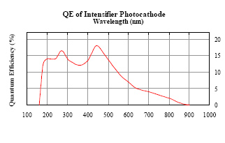
The quantum efficiency of this device is shown in the adjacent figure. The DEP-supplied device has an inherent capacitance (CHPD) of 200 F and provides a gain factor of 2700 at the HV of 12 kV and additionally requires 40 - 80 V bias to collect the electrons across the diode junction. Built into the package is a transimpedance amplifier with 50 kΩ || 1.5 pF feedback, requiring ±5 V supplies. The amplifier circuit also contains a 51.1 Ω resistor in series with the output. Reading out the HPD signal from the amplifier with 50 Ω termination creates a factor of two (50 Ω/(50 Ω + 51.1 Ω)) on top of the 50 kΩ current to voltage conversion.
Frequency Response
Based on the circuit described above, a two-pole response model was developed of the form:
where the parameters in the gain pre-factor (g(ω)) are:
The subscript 'F' in the above expressions stands for op-amp feedback components. G is the gain-bandwidth product - nominally 1.6 GHz but was adjusted to 21 GHz to produce physical results. (Applying this response to the measured responses of LED pulses with the narrow nominal bandwidth produced negative LED intensities!)
The HPD response in the time domain is a straightforward inverse Fourier Transform:
where
Thus, in the complex space, this integral is equivalent to the residues of two poles. Depending on the constants provided, the poles are situated either on the positive imaginary axis or along the -ib/2a line. For the physical constant of our circuit, the former set of poles is relevant. The resulting response function is:
Since the response seen on the HPD circuit output is the convolution of the light pulse shape (fL) with the response function of the HPD, the pulse shape can be recovered by deconvolving the measured signal (fM) with the g. By the convolution theorem:
This is a delicate procedure, in practice, as the division is sensitive to the small high-frequency errors. Direct application of this results in very noisy results. A good remedy is a low-pass filter on the spectrum of the measured signal (taking care to preserve the shape of the signal by keeping the cutoff well above the highest relevant frequencies).
Modeling the HPD spectrum
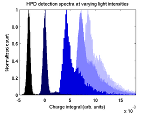
The HPD spectra collected from large pulses should essentially be a convolution of the Poisson distribution, in the limit of high mean count, with the electronic noise function, which is known to be broad enough to make individual photon peaks impossible to resolve. Both of these functions are Gaussian and the result should be a Gaussian as well. The measured spectra, however, show a peculiar deviation (shown on the right.) Clearly, because individual photon peaks cannot be seen with this device and given the large number of photons incident on the HPD window, these cannot be discrete photon peaks. Note also the the shift of the spectrum with increased intensity. Additionally, measurements showed on scaling of the distance between peaks with the gain (adjusted by varying the high voltage bias on the device.)
Our proposed explanation involves ions ejected with some constant probability upon the incidence of accelerated electrons. This positive ion is accelerated in the opposite direction to the path of the electron, back to the bialkali layer. Collision with this layer generates more electrons, which are accelerated and multiplied just as the first. In this model, the lone primary peak of a single photo-electron (h1 of width σ1) is joined by another centered about some value p (of the form h2 with width σ2) representing the mean number of electrons generated by the ion's collision with the bialkali layer. The ratio of integrals of these peaks (α) represents the probability of the ion's ejection for every primary photo-electron. Increasing input to m photo-electrons essentially means a convolution of this spectrum with itself m-times.
This implies a distribution in the total collected charge q from m primary photo-electrons, summed over all possible values of m weighted by its Poisson distribution:
Where fm is the m-times self-convolution of the original primary and secondary peaks of the form:
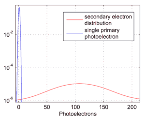
A fit of this model to the data was attempted, assuming the initial peaks are Gaussians, with all parameters remaining free except the gain and the position in the spectrum corresponding to zero photo-electrons. It turned out, however, that the model could not account for the long right-hand tail of the distribution, seen in the above figure. Evidently, the naive assumption that the secondary electron emission spectrum generated by the ion is inaccurate. A crude introduction of asymmetry in the peak of secondaries was introduced by another Gaussian with its location (r), normalization (β) and width (σ3) as another set of free parameters.
Thus the three Gaussians generating the two initial peaks are defined as:
where
Since:
Then, expanding the fm product using the Binomial Expansion, the distribution becomes
This model showed good agreement with the data. The fitter, without any constraints on the third Gaussian, pulled toward a solution in which the peak of secondaries showed slight asymmetry, biased to the left in the spectrum.
Results
The corrected distribution of secondaries, made up of two Gaussians to account for its slight asymmetry, allows the model to fit the measured spectra. First, the following parameters were fixed from HPD/amplifier specifications and no-light distribution ("pedestal") measurement:
- Total gain, including amplifier and oscilloscope waveform mean rescaling: 1.9264 × 10⁵ V/p.e.;
- Pedestal position: -3.6606 × 10⁻³ V;
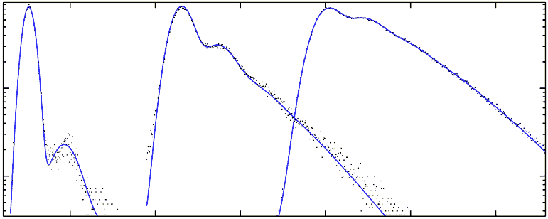
The parameters relating to the shape of the primary and secondary electron distributions, as well as an additional Gaussian noise factor (σ0) were allowed to vary. A fit with these degrees of freedom was performed on three distributions from drastically different light levels (corresponding to roughly 64, 530 and 973 primary detected photons.) The following model parameters produced reasonably good fits (χ2<2.0) for all three distributions.
|
Widths of primary peaks and overall noise:
| ||||||||||||||||||||
Fits with far better agreement were found when the above-listed parameters were free to vary individually for each distribution. Similar and more drastic problems occurred when the simpler one-Gaussian model was used for the distribution of secondary photo-electrons. Evidently, the inaccuracy in its shape is compounded with more convolutions necessary in the high-photon count spectra. Thus, we suspect that the two-Gaussian approximation of this asymmetric distribution is yet not full adequate. However, this already computationally-intensive model (note the three summations) will be even more difficult with more Gaussian and intractable for an arbitrary shape since the convolutions will no longer be straightforward. Disagreements between the fit and data in the right-hand tails of the spectra may also be due to the truncation of the summation in n corresponding to the number of peaks present due to the convolution with primary and secondary distributions.


![{\displaystyle f_{m}(q)=\left[h_{1}(q)+h_{2}(q)\right]\otimes \left[h_{1}(q)+h_{2}(q)\right]\otimes \,\ldots \,\equiv \left[h_{1}(q)+h_{2}(q)\right]^{\otimes m}}](https://wikimedia.org/api/rest_v1/media/math/render/svg/6604cca4af4e9883806f03b0efba07b8c86a0d49)


