

In this web page you will find:

To generate the initial state file all you have to do is edit file decayt.dat (it is in the same directory as mcwrap itself). You have to enter the number of the events of each type you want to generate. For example suppose you want 50000 events Phi->A0 Gamma. You find in decayt.dat the line that names this reaction:
Phi goes
to A0 gamma, A0 goes to Eta Pi, Eta goes to Gamma Gamma.
NNN
... Bunch of numbers you shouldn't care about...
The NNN is the number of events of this type that will be generated. You set it to 50000; you do the same thing for all the events you want to generate. THE EVENTS YOU DON'T WANT HAVE TO HAVE NNN=0!
There is another possibility-you can specify the kinematics after you start GEANT. To learn how to do it go to gradphi++.x". This option maybe useful if you want to calibrate the detector or just look at an event that is too simple to worry about mcwrap.
mcwrap-simple event generator written by Scott Teige. One sentence instruction on how to use it is given above. If you need more detailed instructions you can look in this short manual.
name.itape-this is the file that contains initial kinematics in the form of mc_event groups. Of course "name"-is the name you specify when calling mcwrap with -c option. NO SPACES AFTER -c! The name can be anything you want. If you want to look at the kinematics (say, to make sure it is correct) you can do it with the help of the program dimpEvent, but AFTER you've finished the simulation because this program will look for such groups as cpv_hits etc. It will print contents of these groups as well, event after event.
events.in-the simplest file in the whole simulation. It contains one string that reads "name.itape"-name of your initial kinematics file. DO NOT TYPE ANY SPACES BEFORE THE NAME . After the name hit ?CR>-otherwise GEANT will not open the file. I don't know why but it simply works this way.
decayt.dat- contains specifications of the reactions to be tracked. It uses a special format described in this manual. For a one-sentence instruction look here.
gradphi.x-batch version of the simulation. To run it you just have to type its name in the command line-provided you've compiled it first of course. To compile it just enter make gradphi.x in command line. IMPORTANT: to tell GEANT how many events you want it to simulate you should enter this number in the file controls.in. Namely, there must be a string that says TRIG NNN where NNN is the TOTAL number of events you want to generate. It must be equal to the sum of all non zero numbers of events you have entered in decayt.dat.
gradphi++.x-interactive version of the simulation. To compile it enter make all in command line. It does the same thing as the batch version does but allows you to enter the commands interactively. For instance the command TRIG NNN you had to enter in controls.in described in the previous section you enter at the command prompt. Now, however, NNN does not have to be equal to the total number of events to be generated as specified in decayt.dat. You may enter whatever number you want, but if it is greater than the one in initial kinematics file GEANT will fail over to interactive mode after it generates all the events it knows about. In practice it will mean that after the maximum number of "known" events is reached GEANT will initialize kinematics to zero and track all the rest events as empty-no big deal, just lost of time.
Another option-load kinematics
interactively. To do it you type:
kine
number id energy theta phi vx vy vz
where:
number-number of the
kinematics entry. 1 if you have one entry.
id-particle id for
GEANT as specified in this
manual. Look section CONS300.
energy-energy of the
particle.
theta,phi-polar angles
of the momenta of the particle.
vx,vy,vz-initial position
of the particle.
In this notation 2 GeV photon with its moment along z-axis at the origin will look like this:
kine 1 2 0 0 0 0 0
This is useful if you, say, want to calibrate the detector. When I calibrated it I shot 1 GeV photon inside the LGD and demanded that the sum of the energies detected by all LGD blocks equals to 1 GeV. This procedure, if you do it several times and plot the resulting histograms, also gives the resolution curve of the detector. For an example look here.
simData.itape-the output file that contains such structures as cpv_hits, lgd_hits, upv_hits etc for each event tracked. In the beginning of each event there is also group mc_event that contains the kinematics for this event. It may be useful for future analysis. The file is ready to be analyzed by the standard methods for Radphi. It does not have to be unpacked-GEANT does it for you.
your
analysis-it is whatever you want
to do with the simulated data. Anything that understands *.itape files
will understand the output file.
Suppose you want to generate
10000 events Phi->A0+Gamma. You should do the following.
The first 0 after the title is the
number of events to be generated. Set this to 10000.
PhiA0Gamma is just a name of the
output file. You can choose any. This command will create the file PhiA0Gamma.itape
in the mcwrap workind directory. You should move it to the directory ../Gradphi/
where it will be accessible to GEANT.
No spaces before
the name!
This will tell
GEANT to generate 10000 events.
Below you can find some example of
the use of the presented Monte Carlo simulation. Fig.1 is the ray traced
view of the detector with the herculite cover removed. If you look hard
enough you may actually see the target near the center of the RPD. It has
almost the same color as the light guides but it has to do with the density
(I didn't choose colors otherwise the target would be much better visible).
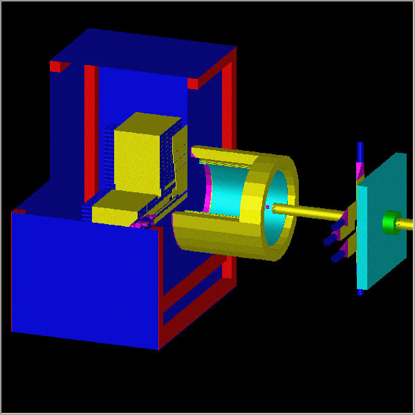
Figure 2-logical tree of the detector. Each blue box represents one logical element. Names are marked in yellow (don't worry if the names seem weird; they are internal GEANT names and user doesn't need to know them). You may notice that the tree looks simple even though the detector itself is quite complicated. The simplicity of the tree allowed to reduce the tracking time down to 300 ms per event.


The following figure contains information about the resolution of the detector. It was obtained by shooting 0.3, 0.6, 0.9, 1.2, 1.5, 2 and 4. GeV photons and measuring the corresponding width. The fit is miraculously close to the published result for detectors of this type, namely


Next two plots
obtained by generating 65000 events of the type Phi->A0+Gamma
and Omega->Eta+Gamma respectively. On the
first plot you can see invariant mass of all five-cluster events. The second
plot contains invariant mass of all two-cluster events. The peeks are located
remarkably close to the actual masses of Phi and Omega respectively. No
recalibration has been applied!


exec mctuple simData.itape [count=NNN]
count-number
of records to be read. If absent all records are read. This will
load the ntuple into memory. After this you can work with the ntuple as
usual.
If you have any questions or comments
please contact Andriy Kurylov.