X-ray Rocking Curve Analysis
Richard Jones
started June 20, 2019
Table of Contents
other instrumental artifacts 17
horizontal beam divergence correction 28
independent d-spacing extraction 30
errors on the extracted (1,0,0) surface shape 34
new systematic: complementary image distortions 35
Comparison of virgin samples from cls-11-2017 54
June 20, 2019 [rtj]
We now have accumulated a large number of X-ray rocking curve topographs of our GlueX diamond radiator inventory, but so far we have not fully explored what these rocking curves are telling us about these crystals. Here are some unanswered questions whose answers may lie hidden in these data.
Subsidiary to these larger questions are more specific questions related to the quality of the rocking curve data and the systematic errors associated with extracting crystal properties from the measurements.
I will attack these questions in reverse order because the quality of the answers to the questions in part A depends on the answers from part B.
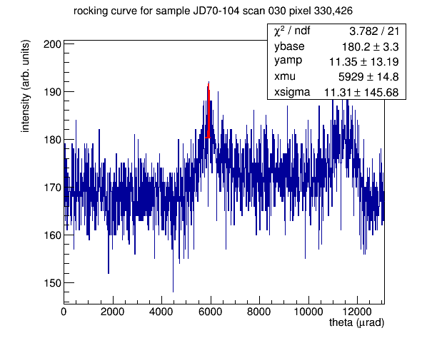
We use as small as step as we can in the Bragg angle when doing rocking curves in order to get the best resolution possible on the rocking curve profile. When we were working at CHESS, there was no problem advancing θ in steps of one arc second (5 urad) or less at a time. But at CLS the stepper motor we are using for θ has a single step size of 0.72o (12.57 mrad) and a main screw pitch of 1.667 revolutions of the motor per degree θ, leading to a θ step size of 21 urad. This is an order of magnitude more coarse than we need in order to resolve the rocking curve width, so we set up the stepping motor to use 250 microsteps per 0.72o step, or 0.00288o per microstep. This allowed us to take a rocking curve image every 0.00014o in a continuous scan through the diffraction peak, or one image per 29 microsteps. This was the setting for all of the scans we took in the June run, 2019.
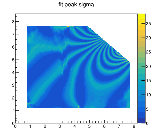
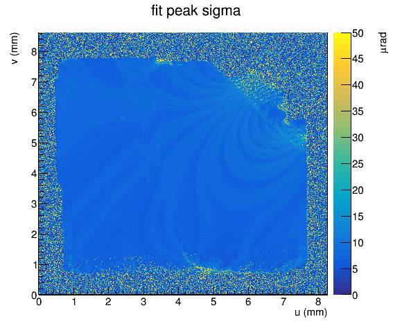
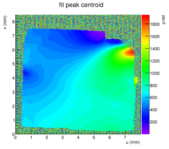
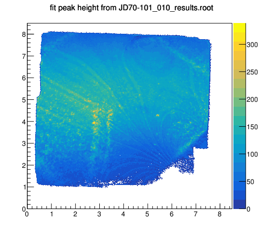
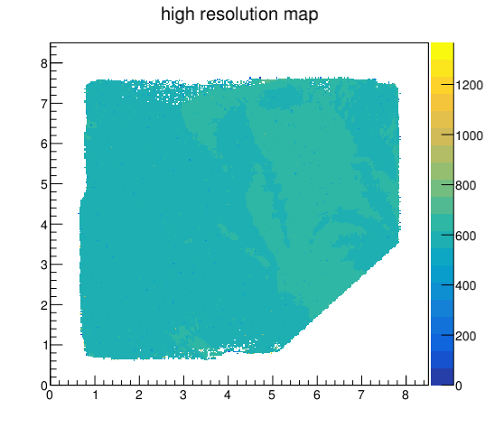
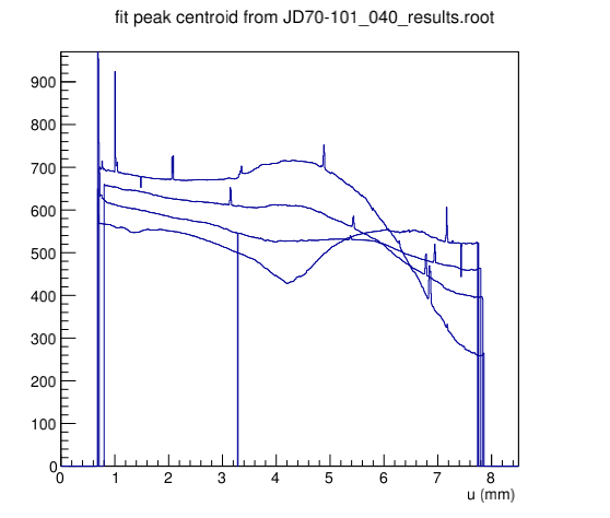
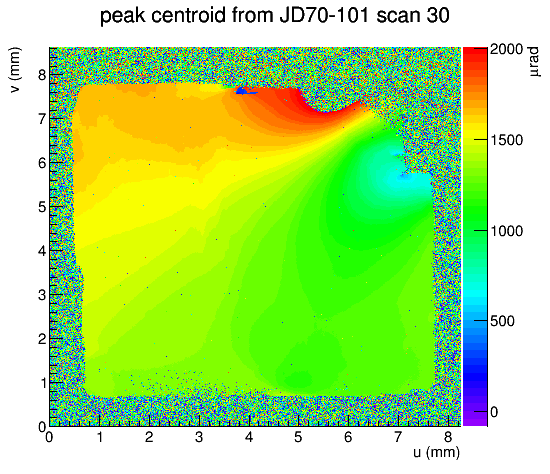
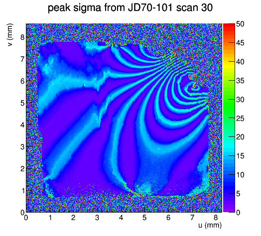
Although this looks good on paper, the motor did not advance at a uniform rate each time we stepped forward these 29 microsteps. Sometimes it seemed to not advance at all, and other times it stepped forward by much more than 0.00014o, in something that resembled a saw-tooth pattern. This pattern is imprinted on the measured rocking curve width topograph, as shown in the image below taken from one of the first scans taken of JD70-101 during the June, 2019 run.
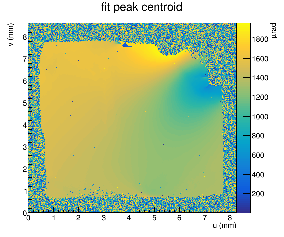
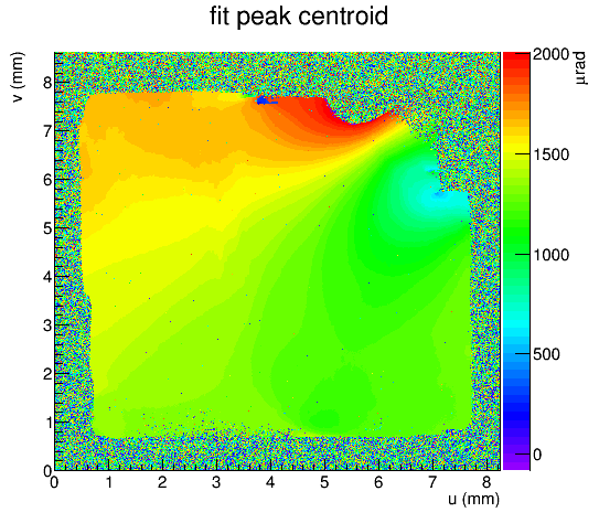
In this image, the high ridges indicated by the light blue color indicate the pixels that were near their diffraction maximum when the motor stopped advancing, giving the appearance of a broad rocking curve peak. Conversely, the low valleys indicated by the purpose color identify pixels whose diffraction maximum occurred during a part in the scan when the motor was advancing faster than average per step, giving the impression that the peaks are narrower than their neighbors. The fact that this same pattern appears on every scan of diamonds that have been untouched by radiation damage, and that the ridges and valleys follow the contours of equal Bragg angle (see plot at the left) together indicate that this is an artifact of the θ motor.
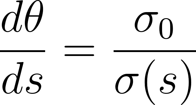
As a first approximation, I consider that all of the pixels outside of a triangular region in the upper right corner of these images have the same rocking curve peak sigma. Under this assumption, one obtains Eq. 1 for the motor step size dθ/ds as a function of step number s.
(1)
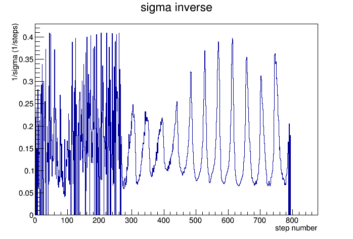
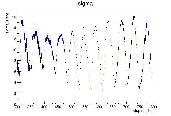
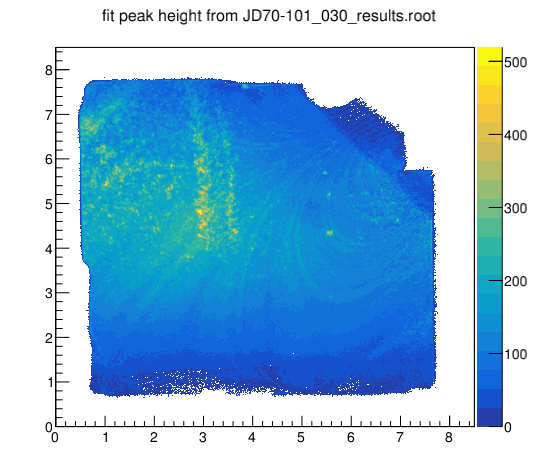
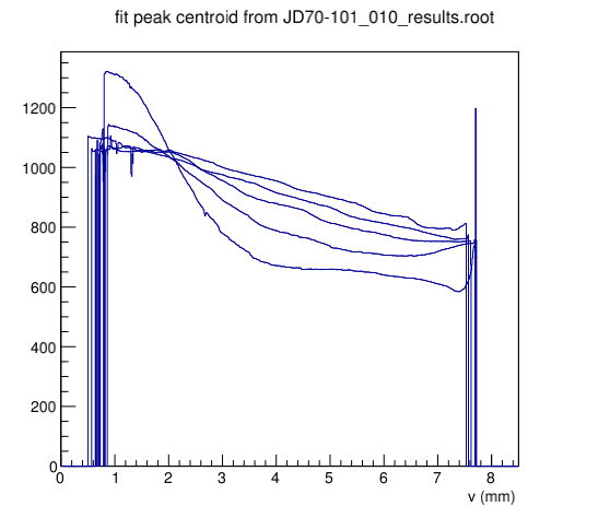
where σ(s) is the measured mean rocking curve width for pixels that reach a maximum at step s, and σ0 is the true (average) rocking curve width for those same pixels. I don’t know the value of σ0 from first principles, but I can obtain it from the constraint that the average value for dθ/ds must equal the nominal value from the logbook, 0.00014o or 2.443 urad per step. The function 1/σ(s) for scan 30 of JD70-101 is shown below.
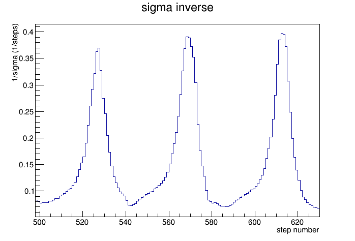
The lower plot above is the shows the same data as the upper one, zoomed in on the x axis.
Normally one would expect a cyclic machine like a screw-cog system to exhibit periodic nonlinearity. The fact that the period is the same across the entire sample but the amplitude of the oscillations is changing suggests that there is something missing from my model having to do with the assumption that the average rocking curve width is constant across the scan. At the start of the scan, the pixels are all grouped in the lower half of the chamfered corner. At the end of the scan they are all grouped in the upper half of the same corner, but that end gets cut off by the mask that I placed over the sigma plot to avoid bad regions of the crystal. But it is clear that I do not fully achieve this avoidance, as evidenced by the fading out of the oscillations into noise at the early end of the scan. A similar fading out appears to be taking place at the late end of the scan, right before the sequence is cut off by the mask. The mask cut is shown by the fact that the fits stop before step 800, whereas the peak centroid plot above shows that fits continue to find peaks in the upper right corner of the image right up to the end of the scan range at step 878.
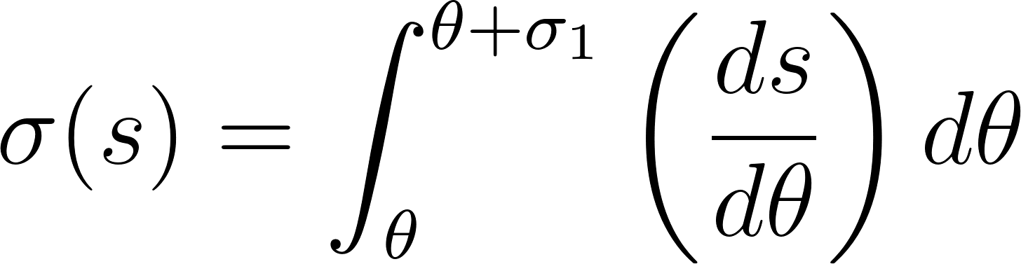
How would an increase in the intrinsic rocking curve peak width over its minimum value σ0 change this analysis? In Eq. 1 I assumed that the peak width is much smaller than the scale of variations in dθ/ds so that the slope of θ(s) is assumed to be constant over the width of the peak. What if the peak width approaches the scale of the period of the motor nonlinearity period of 42 steps? Then Eq. 1 needs to be replaced with Eq. 2, where σ1 is the enlarged peak width, relative to the ideal minimum value σ0 for this crystal lattice vector and energy.
(2)
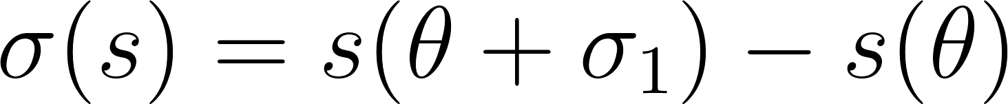
This turns into Eq. 1 when dθ/ds is a constant within the width of a peak and can be brought outside the integral. To go beyond the constant-slope approximation, let me treat dθ/ds as a sinusoid with a dimensionless angular frequency ω.
(3)
where s(θ) is the integral of ds/dθ from the start of the scan. Let ds/dθ = s0 + s1 sin(ωθ), then
(4)
Eq. (4) shows how the effect of Eq. 1 is attenuated as the peak width σ1 broadens. For example, if σ1 = 2π/ω then the second term in Eq. 4 is zero, and the measured width σ1 receives zero correction from the nonlinearity. Only in the limit σ1 << 2π/ω do the corrections approach those given in Eq. 1.
For small peak width ωσ1 the second term on the last line in Eq. 4 is of order (ωσ1)2 and the third term is of order (ωσ1)3. The second term produces a shift in the maxima of the oscillating function σ(s), while the third term decreases the amplitude of its oscillations. I clearly see the decrease in amplitude at the two ends of the scan in the above inverse sigma plot, so is there also a deviation from regular spacing between the peaks in those regions? Here are the step numbers of the maxima in the above figure.
There is 10% in the peak spacing across the scan, but that is not enough to explain a 50% change in the modulation amplitude of the function σ(s). However, there is another reason why the first correction in Eq. 4 might drop out, leaving the second correction as the leading effect. The reason for this is as follows. Eq. 2 only gives the correct answer for the fitted peak width σ(s) if the peak is symmetric, so that the same answer is obtained with the replacement σ1→-σ1 and -σ(s)→-σ(s). If the peak is asymmetric, the fit will give something close to the average between the left and right side HWHM distances from the peak maximum. Examination of Eq. 4 shows that the zeroth-order and second-order corrections do not change sign under this reversal, whereas the first-order correction does. Therefore it should drop out if one uses the fitted peak width to estimate σ(s). On the other hand, this term will produce a shift in the fitted peak position which one may want to take out at some point down the road in a comprehensive treatment of this effect. For the moment, I simply want to check that I can extract the function ds/dθ reliably from these data.
From now on, I look directly at σ(s) instead of its inverse, and try to build a model for ds/dθ out of it, based on a few assumptions.
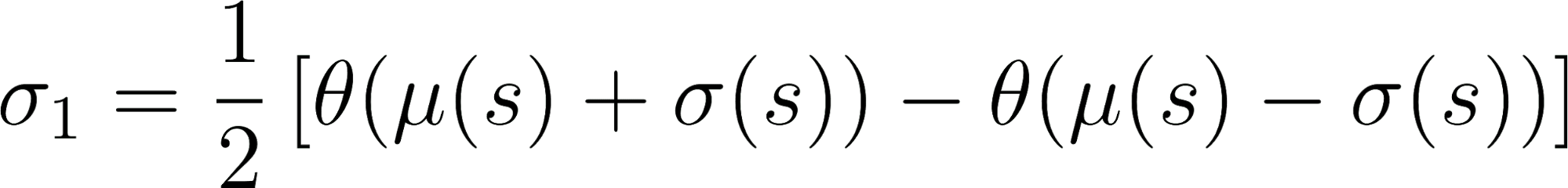
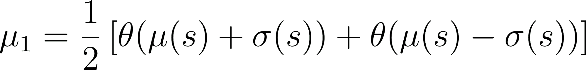
A symmetrized version of Eq. 3 is needed to see how to extract a corrected peak width σ1 and peak centroid μ1 from the measured width σ(s) and mean μ(s) of each pixel.
(5)
(6)
where the function θ(s) is the inverse of s(θ) that is obtained by fitting and integrating ds/dθ. In Eqs. 5,6 the measured peak centroid μ(s) and width σ(s) would vary depending on the phase of the motor at step s, but the corrected centroid and width μ1,σ1 would not.
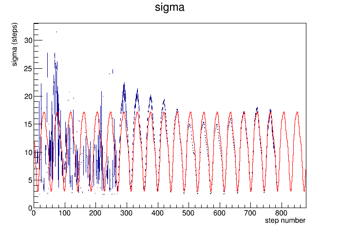
The next plot shows the function σ(s) extracted from JD70-101 scan 30. Notice that superimposed on the regular periodic motor nonlinearity there is a modulation that moves through the peaks, making the leading edge steeper on the left and the trailing edge steeper on the right. I will not try to capture this behavior in full detail initially, just take a smooth periodic shape that approximates an average of the cleanest central 4 peaks, and see where that leads.
The above curve in red is a periodic function with a period of 43 steps, expressed as a Fourier series with a fundamental plus 4 higher harmonics. The coefficients are listed below, in the order cosine, sine.
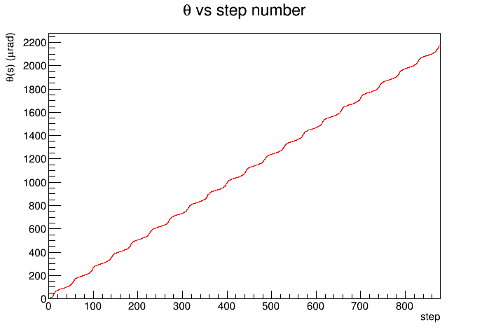
I now rescale this periodic function so that its average equals the 0.00014o per step nominal step size for the rocking curve scans in this dataset, then integrate its reciprocal to get θ(s) for use in Eqs. 5,6.
The corrected results for JD70-101 scan 30 are shown below.
There is still a residual stripe pattern visible in the sigma plot left over from the motor nonlinearity, but for the most part the effect is removed and the true rocking curve width is now discernable over the entire active area of the crystal, somewhere between 10 and 12 urad.
June 26, 2019 [rtj]
Today I want to go ahead and form similar corrections for all of the scans we took at CLS during the June, 2019 run. The motor-corrected topographs named hmu_moco and hsigma_moco are saved the the JD70-XXX_YYY_results.root file, alongside their uncorrected siblings.
I completed the above operation for all of the scans except those of JD70-104, the 20 micron framed diamond. I did not apply the “moco” correction to those because the total width of the scans are so large that there is insufficient resolution to fully separate the motor modulations, and at any rate the motor modulations do not make much difference when the peak width is dominated by radiation damage.
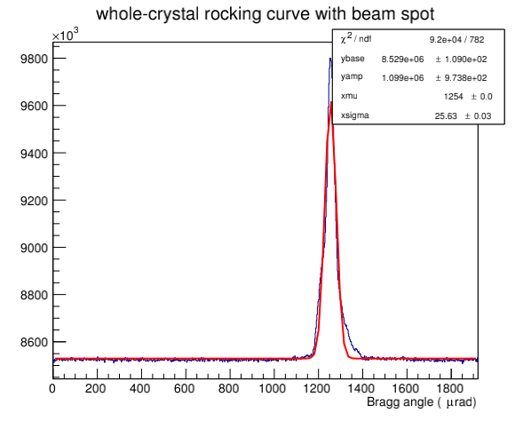
Before I move on, I want to develop one more bit of functionality: the ability to select a region for a beam spot and generate a whole-crystal rocking curve weighted by the local beam intensity. For this I would like to have the ability to select the center of the spot using the mouse and have the integrated rocking curve generated based on that spot.
June 24, 2019 [rtj]
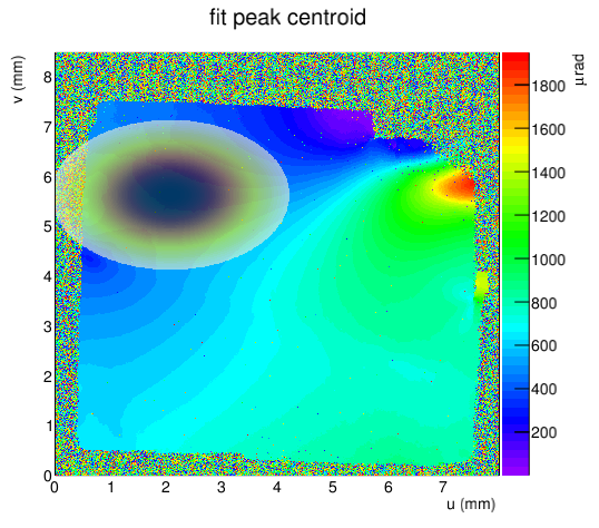
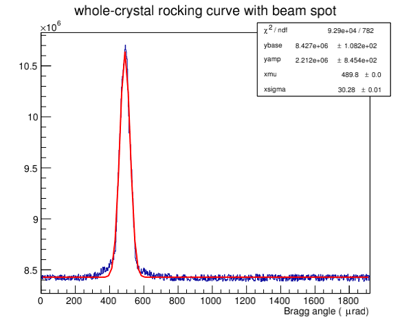
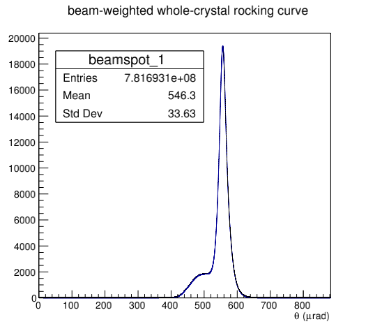
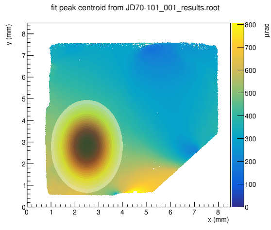
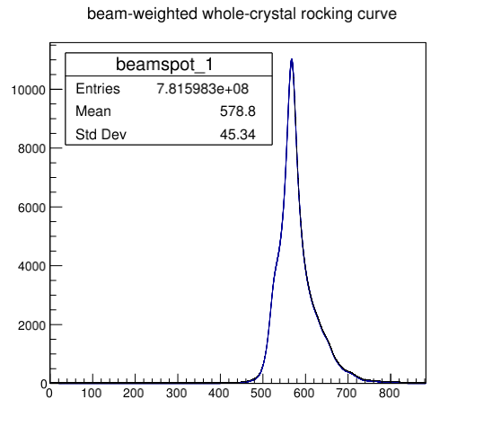
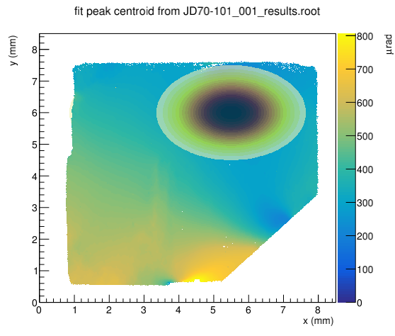
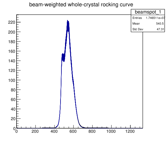
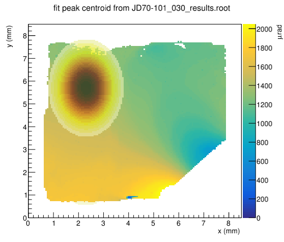
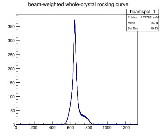
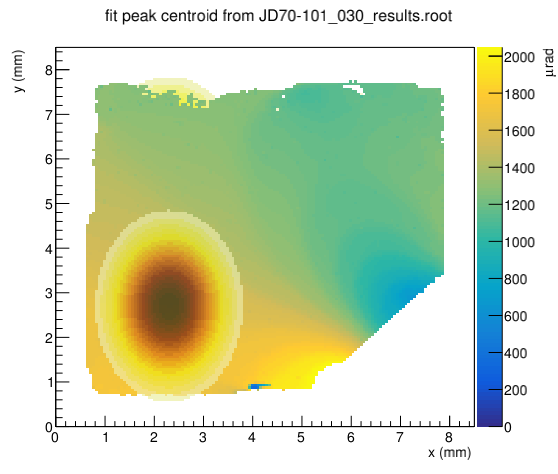
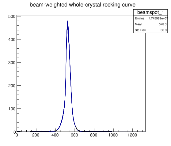
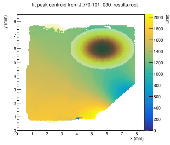
Below I show the first results from a new program I wrote for this purpose, beamspot.C in ~www/docs/halld/diamonds/Analysis. The original rocking curve mean topograph for scan 30 of JD70-101 in run period cls-6-2019 is shown first. The second plot is a copy of the first, with an image of the beamspot gaussian superimposed at the position selected by a click of the mouse. The third plot is the whole-crystal rocking curve weighted by the beam spot intensity.
Rocking curve topograph for JD70-101 scan 30, with a user-selected beamspot superimposed.
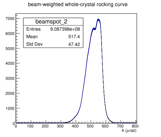
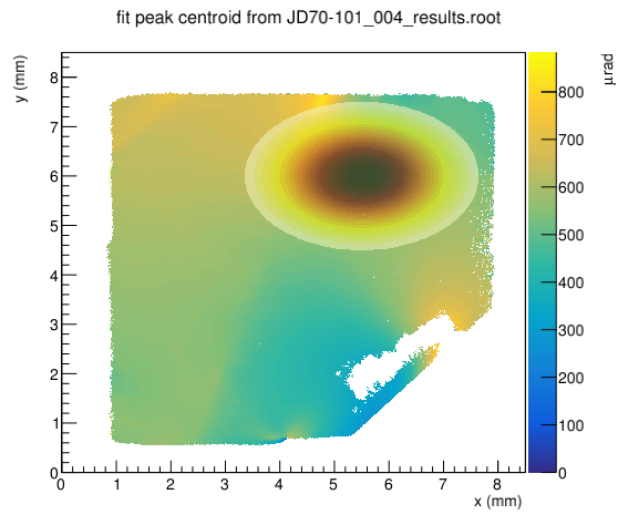
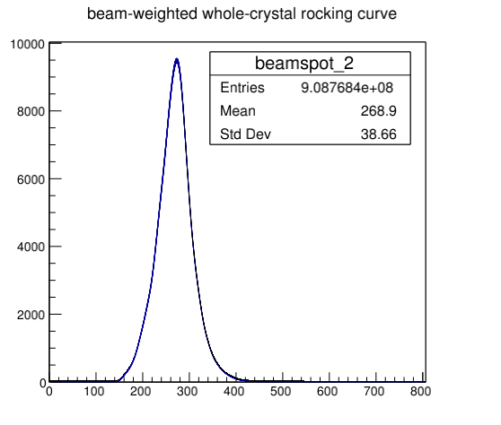
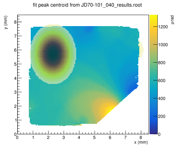
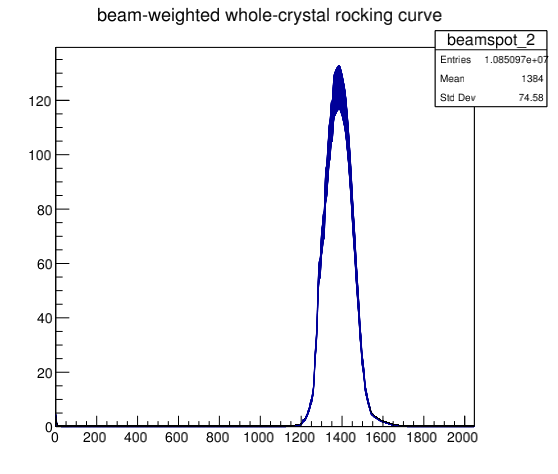
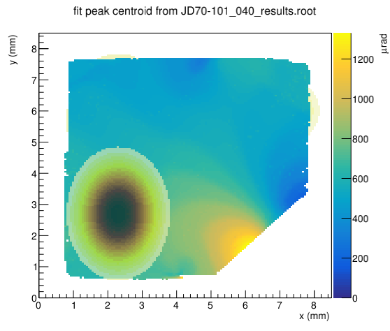
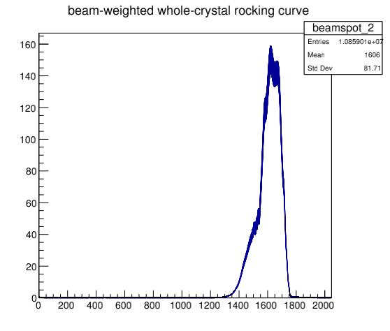
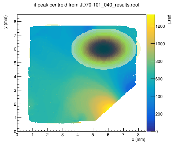
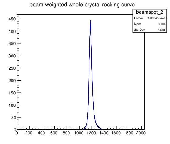
The plots below show the same sequence of plots, this time for JD70-101 scan 40.
In both cases, the beam-weighted rocking curve width just about matches the Gluex design spec of 20 urad sigma.
June 26, 2019 [rtj]
A number of the rocking curve topographs that were taken during the June 6, 2019 run have ragged edges along the bottom and/or the top of the crystal, as a result of the limited height of the BMIT X-ray beam, and the imperfect vertical placement of the sample within the beam envelope. Today I thought that perhaps it might be possible to extend the set of fit-able pixels by combining adjacent sets of images together and reducing the scan resolution. I tried this on JD70-106 scan 10, which had drop-out pixels along both the top and the bottom edges of the crystal. I makes no sense to rebin the scans in steps wider than the single-pixel rocking curve width because that just makes the signal/noise worse within the peak. It was a surprise to see that I could not get any improvement in the fraction of fit-able pixels in the low-intensity regions of the crystal by this kind of rebinning technique. The additional noise introduced by the rebinning had a greater effect than the increased signal obtained by summing.
In the future, we may want to take multiple snapshots at each step. In this way we would be able to average the noise without any loss of signal. But given the data we have, there is not much more that can be done than what the rcfitter is presently giving.
June 27, 2019 [rtj]
Before I can combine different scans of the same diamond in a combined analysis to extract geometric properties of the crystal, such as the d-spacing and strain profile, I need to rotate, invert, and shift the images so that the different images are aligned. The question to be answered first is, to what degree the position and angle of the diamond can be extracted from the measured topographic images.
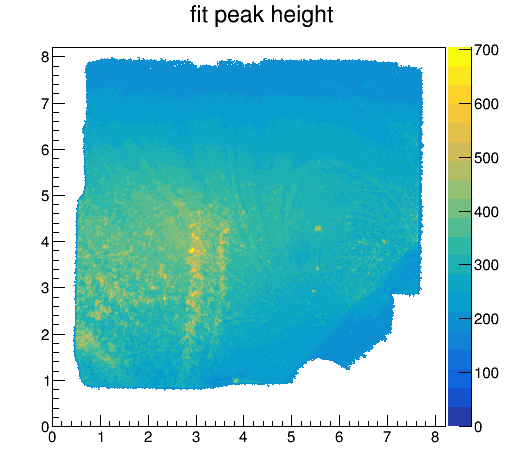
Edge detection in these noisy images is a real challenge. For starters, I look at the hamp map, illustrated below. The left image is JD70-101_10 with the edges cleaned up using the function plotgen.get_silhouette, whereas the right is JD70-101_30 with a similar cleanup applied, followed by a Rescale(1,-1,1) to flip it vertically for direct comparison with scan 10.
Similar features are seen in the two images, but there are differences that make it a challenge to align them, including:
All we really need to complete the alignment is two points that can be identified between the two images. I wonder if I might do the alignment manually by selecting two local maxima with a mouse and have the analysis software locate the maxima as precisely as possible in the two images and perform the appropriate rotation + shift to bring the second image into registration with the first.
I implemented a dynamic alignment function in plotgen.py named dynamic_align which displays two topographs rapidly, alternating between the two in the same canvas, and accepting suggestions to nudge the second one right/left/up/down/clockwise/counter-clockwise until the two images show no more shift as the user flips quickly between them. This worked quite well for aligning JD70-101 scans 10 and 30 which are 180o away from one another. There are two bright spots visible near the middle of these two intensity images that were fairly easy to force on top of one another. It is gratifying to see that the distance between them is sufficiently close that they could be simultaneously aligned just by a combination of uniform shifts and rotations. However, once those two spots are aligned, there is still a mismatch between the two images, as can be easily seen in the animation below.
Even though the two anchor points are not shifting significantly, there is a clear difference in the skewness between the two. I have the impression that the difference visible here could be removed by a shear transformation that shifts the top of the h30 (darker at the top) image left while shifting the bottom of the same image right (brighter at the bottom) while leaving the central part of the image unchanged.
Moving on to orthogonal pairs, I now try dynamic alignment of scans 10 and 40 for JD70-101.
Here the match is much better than what I obtained before between scans 10 and 30. There are slight differences in the exact edge shapes, but I think it is going to be very difficult to do better than this. Lastly, I try the same thing between scans 10 and 50.
Once again, there are slight differences in the detailed shapes of the two edges, but overall the alignment is visually quite good. Perhaps with further manual effort I could do marginally better, but at some point one runs into the limits of the optics of the camera and projection geometry.
The alignment is now pretty good. But I wonder if I might do a little better with some sort of automated procedure. Apart from the 45o chamfer, the edges remain the best overall guide to image alignment.
To get the quality of the alignment shown in the animated plots above, I needed to adjust the aspect ratio of the images by a small amount. In the case of scan 10 - 40 alignment, I had to expand the width of the scan 40 image along x and decrease it along y by a factor 1.0125, for an overall increase of the aspect ratio of 2.5%. In the case of scan 10 - 50 alignment, I expanded the width of the scan 50 image along x and decreased it along y by a factor 1.0085, for an overall increase in the aspect ratio of 1.7%. I suspect that the true correction factor is somewhere between these two, around 2.1 ± 0.4%. Taking this 0.4% as the relative error on my knowledge of the distance scale in these camera images is a good initial estimate.
So far in my pair-wise comparison of rocking curve images, I do not see evidence of artifacts that cannot be explained as coming from the crystal. If there are such, they will probably show up when I try to extract a consistent set of crystal model parameters from the images. I proceed to do that now.
June 28, 2019 [rtj]
To prepare for coordinated analyses of pairs of rocking curve topographs, I decided to reorganize the various utility functions I have developed in the work described above into a new python class named Couples. A couple relates two rocking curve scans to one another, containing the information needed to overlay one on the other, mask off noise pixels, and make any other corrections needed so that comparisons with geometric model predictions can be made. Various bits from plotgen.py are being moved from there into Couples.C, and new methods added to make the Couples class a robust toolkit for rocking curve analysis. I decided to write it in C++ instead of python so that it fully integrates with ROOT and Couples can be saved as TObjects in a ROOT file. The plan is to create a new ROOT file for each set of rocking curve scans, e.g. JD70-101_couples.root, where the Couples will be saved. Initially a couple will only relate two scans, one from each of the two orthogonal scan directions, but eventually one might want to extract combined information from two complementary Couples that gives information about the differences in model shape from the front and back-side scans, and perhaps about d-spacing changes and other effects that go beyond a simple geometric model of the crystal strain.
July 2, 2019 [rtj]
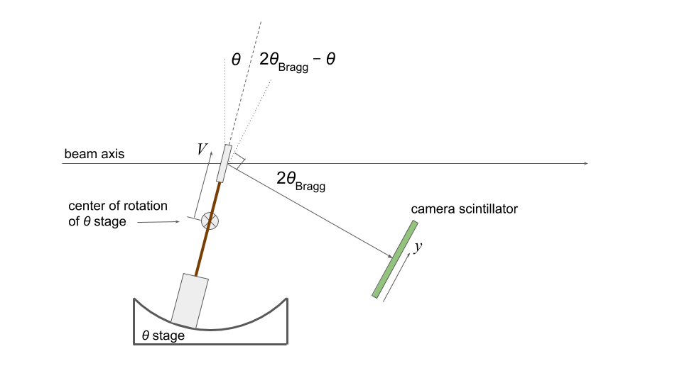
The Couples class is now complete, and I am ready to start analyzing pairs of scans to compare the results with a geometric model of the crystal geometry. Here are the parameters of my geometric model, including the beamline and how the different axes are defined.
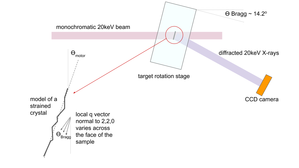
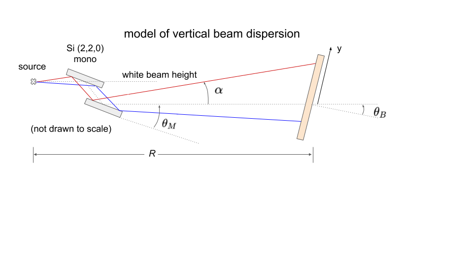
Figure 1. Illustration of the beamline and target geometry showing the parameters of the model.
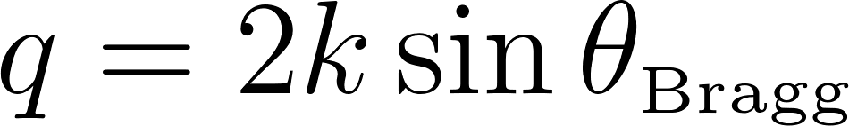
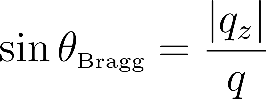
The diffraction condition is
(1)
where q = 9.820 keV is the momentum of the (2,-2,0) reciprocal lattice vector, k = 20 keV, and θBragg = 14.212o. Relating θBragg to the properties of the target and setup entails the application of trigonometry to the geometry illustrated above.
(2)
(3)
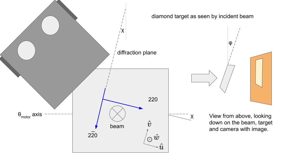
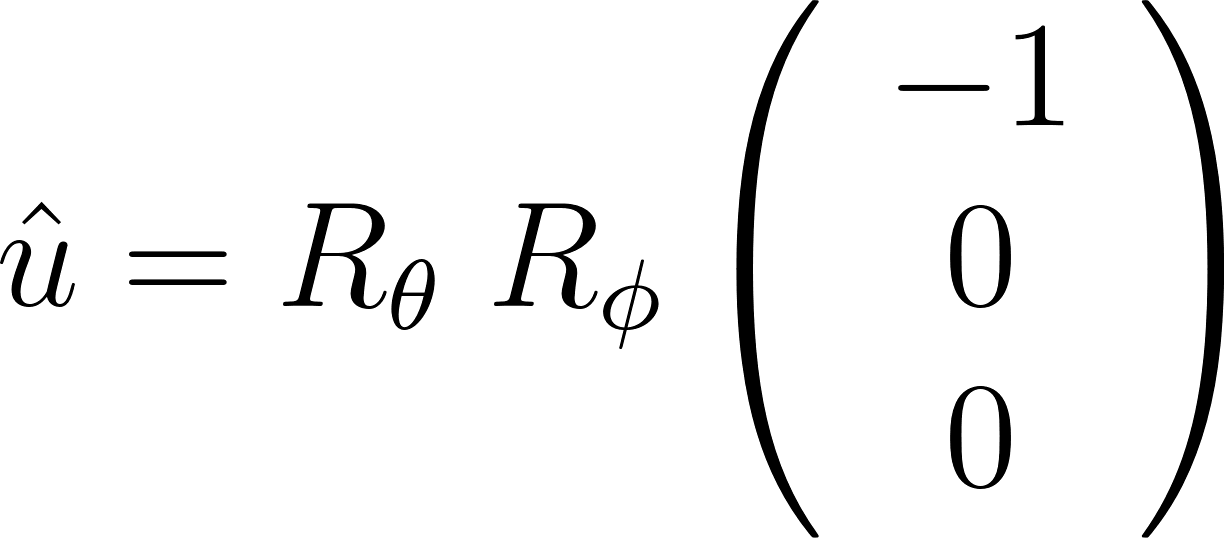
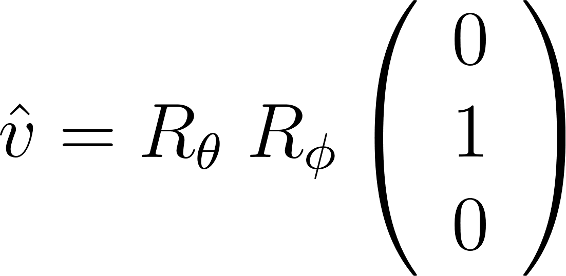
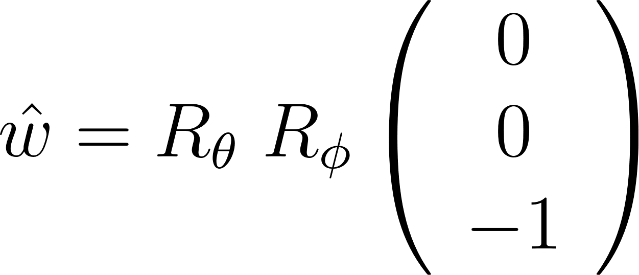
assuming a down-bounce Bragg reflection, where the unit vectors u,v,w form a right-handed coordinate system aligned with the principal axes of the crystal, as shown in the above figure. The θV in Eq. 3 represents a small deviation of the local q direction from the global average for the crystal. The significance of this local variation will become apparent later.
(4)
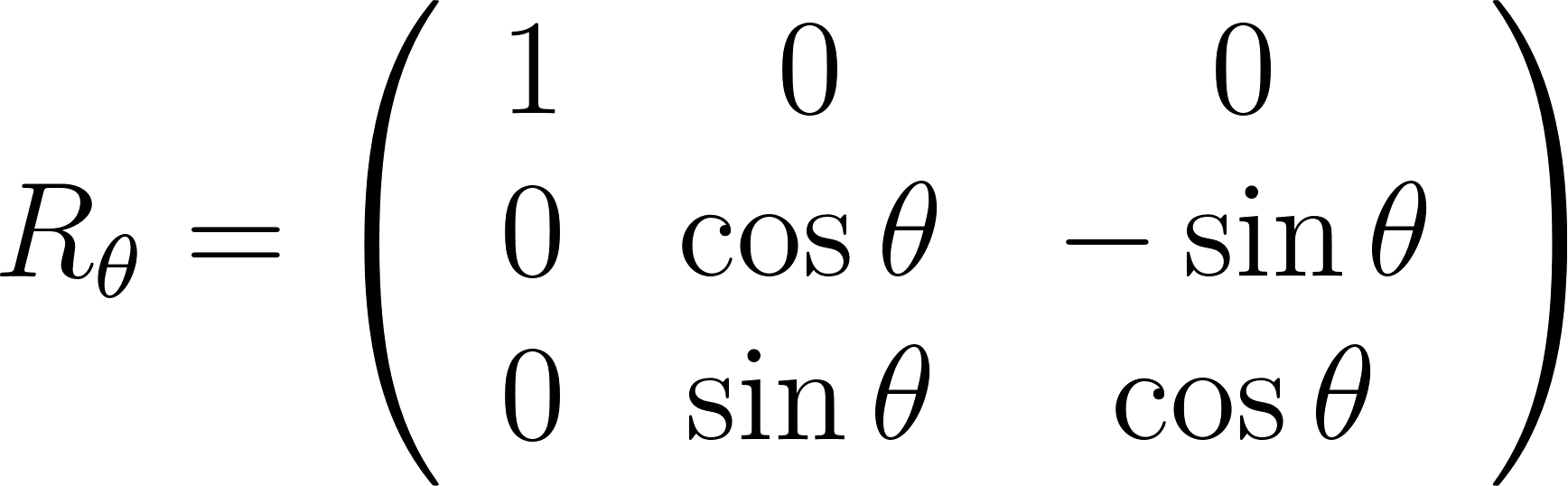
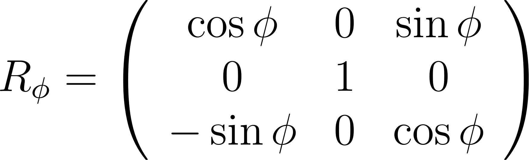
with respect to standard beam coordinates with (0,1,0) pointing up, (0,0,1) along the beam direction, and (1,0,0) pointing beam-left.
(5)
Here a definite order has been assumed for the operation of the three rotation stages. This may be different from the order of the stack that was actually used for the X-ray rocking curve measurements, which in fact probably varied from one run to the next. Here I assume that the angles φ and ꭕ are small enough that their rotation matrices commute. In any case, we do not directly measure their values and they were not varied during the scans, so the order in which they are applied does not matter to this analysis provided that they are not assumed to be zero. Substitution of Eq. 3-4 into Eq. 2 leads to
(6)
(7)
Eq. (7) shows that θBragg = θ for a perfect crystal under ideal alignment conditions θV=φ=ꭕ=0. Further, it shows that variations over the surface of the diamond in the value of θ where the Bragg condition is met are directly interpretable in terms of the local variation of θV . Assuming that the misalignment angles φ and ꭕ are small, on the order of a few degrees, Eq. (7) can be rewritten in the form,
(8)
which shows that θV can be read off directly as the variation in the value of the Bragg rotation stage θ at which the diffracted intensity peaks for each pixel in the topographs. In terms of the crystal geometry, θV is the angle between the local v axis of the crystal and the nominal uv plane of the entire crystal. The rocking curve measurements have an arbitrary offset in the value of θ reported for the Bragg rotation stage at each point in a scan, so the definition of the nominal uv plane entirely a matter of convention. In what follows, I will adjust the nominal plane to roughly level the uv surface, with the understanding that only the shape is measured; the orientation is arbitrary.
To obtain a 3d image of the 2d uv surface, I need to combine the θV information from two different scans, one with the (2,-2,0) axis aligned with the v axis as shown in the above figure, and the other rotated by 90o to align (2,2,0) with v. When we took these measurements we were careful to rotate the sample by 90o between the two scans to within 0.5o or better. With this in mind, I assume that a pair of scans is described by just a single ꭕ offset which must be determined from the data.
Let x,y be defined as the camera image column, row coordinates rescaled to mm in x and rescaled to mm / cos θVBragg in y so that x,y is a Cartesian map of the crystal face. Furthermore, let W(x,y) describe the profile of the uv surface over the crystal face, including all of its non-planar distortions. Note that W(x,y) describes the strain of the crystal that distorts it away from its ideal planar geometry, not the profile of the physical surface; W(x,y) is a property of the bulk crystal, not its front or back surface. Finally, let DU(x,y) describe the local lattice spacing of the crystal along the (2,2,0) direction, and DV(x,y) the local lattice spacing along the (2,-2,0) direction, expressed in units of the ideal diamond lattice constant. These three functions W, DU, and DV express the full understanding of what can be extracted from a set of 4 rocking curve scans. As I show below, the reduction from 4 measured topographs to 3 model parameters comes from the constraint in the model that a fourth function that is interpreted as the curl of the gradient of W should be zero. Verifying this constraint is an important step in this analysis.
July 3, 2019 [rtj]
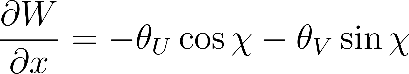
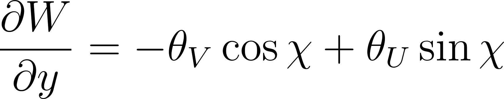
To leading order in small parameters θU , θV
(9)
where θV is measured with the target in the orientation shown in the above figure, and θU is the same thing taken after rotating the crystal counter-clockwise in the figure so that the new u axis points along the direction of the old v axis. For Eq. 9 to hold for a single global function W(x,y), there is a constraint that must hold between the maps for θU and θV arising from the identity that the curl of the gradient of W must be zero.
(10)
This consistency check must be satisfied before the analysis can proceed to the extraction of results for W, DU, and DV. Alternatively, it can be used as a means for estimating ꭕ which is difficult to measure directly with our topography setup.
Once Eq. 10 is satisfied for a realistic value of ꭕ, Eq. 9 can be used to find the gradient of W, and then the gradient integrated to find W. In practice, this last step is complicated by the fact that the measured local values for θV and θU are noisy, so that while Eq. 10 may be satisfied on average over the entire crystal, there are local deviations. A more consistent approach is to use Stoke’s theorem to compute W by integrating the gradient along a closed loop path around the outer periphery of the crystal area in the images, and then solve for W inside the loop using Poisson’s equation, with the W values around the outer loop as the boundary conditions.
(11)
When preparing the W outer loop, I adjust its height and tilt to more or less level the surface, so that the solution can be plotted in a way that makes the non-planar structures most apparent. The technique was anticipated some years ago when I started working on tools for this purpose, and I found all of the methods needed to do this were already a part of the Map2D class. The next section shows the first results obtained using this approach.
July 4, 2019 [rtj]
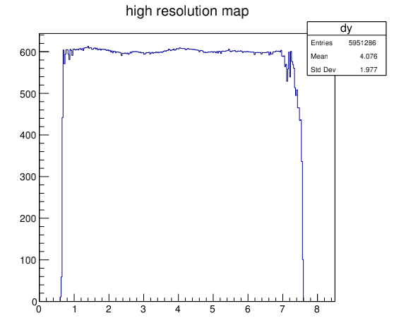
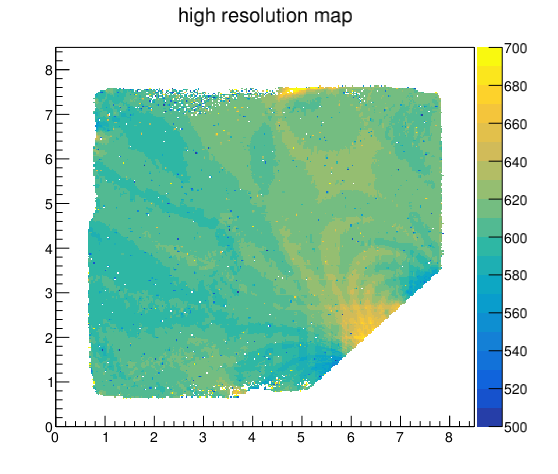
The geometric model described above predicts that two scans of a virgin diamond that are related by a 180o flip around the θ axis should be identical, once the upside-down image has been inverted. However, this ignores the presence of vertical dispersion in the beam. An attempt has already been made to correct for this dispersion in rcpicker::Normalize that is applied to the hmu topograph before it is written to the results.root file. The presence of a vertical slope on the difference plot between such a pair of topographs provides in independent check that the dispersion has been completely removed. If not, residual beam dispersion effects will appear as a spurious curvature along both x and y directions, distorting the shape of the crystal that emerges from the geometric analysis.
The plots below shows a strong residual dispersion effect when comparing scans 1 and 3 of JD70-101. First I show the raw images to show that these two scans are 180o apart. I then show the difference of the two topographs, once the second has been inverted in y and the two images have been aligned.
The residual dispersion is half of the fitted slope parameter, about 20.2 urad/mm in y. This is in very good agreement with the calculated value of 20.5 urad/mm that was encoded in rcpicker.C for the cls-6-2019 run. There are several possibilities here:
In a down-bounce geometry, the y-dispersion should be negative, with larger energies at the bottom of the beam spot, and lower energies toward the top.
July 5, 2019 [rtj]
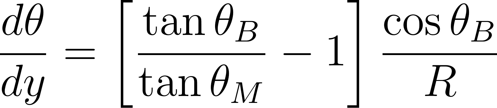
The model I used to predict and correct for vertical dispersion in the X-ray beam is illustrated in Fig. 2 below. The distance from the source in the dipole bending magnet to the target is R. The dip angle (increasing downward) of the X-ray coming from the source relative to the horizontal plane is ꭤ. The angle of the silicon monochromator crystal planes relative to the horizontal is θM and for the diamond crystal is θB.
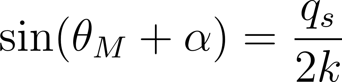
It follows from Eq. 1 that
(12)
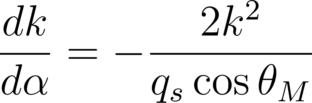
where qS is the crystal momentum corresponding to Si (2,2,0). For small ꭤ, this leads to
(13)
The fact that
(14)
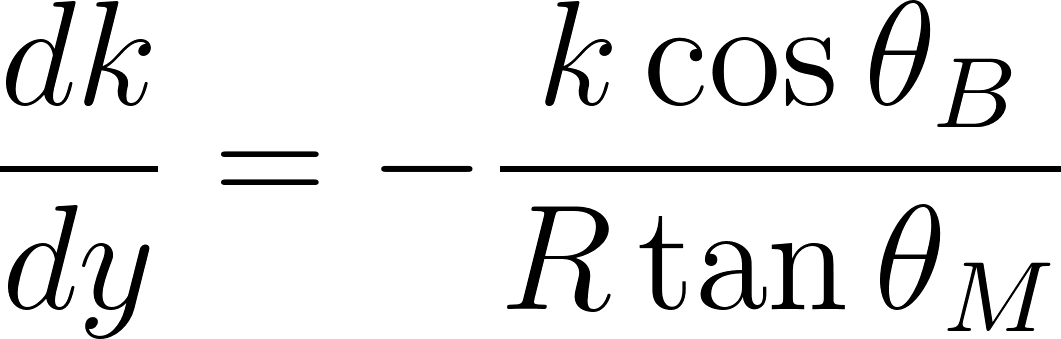
leads to the vertical dispersion over the surface of the diamond given by Eq. 15.
(15)
For an ideal planar diamond, this produces a shift in the Bragg angle θ(y) at which the diffraction intensity is maximized given by
(16)
written in terms of the crystal momentum of diamond (2,2,0) qd . Since qd is constant,
(17)
Substituting dy/dy from Eq. 15 and dꭤ/dy from Eq. 14 leads to the desired result in Eq. 18.
(18)
The value of R for the BMIT beamline we are using is R=26m, and at 20 keV θB=14.2o, θM=9.29o, leading to dθ/dy = 20.4 urad/mm.
The next question is, was the correction applied correctly during the initial fitting procedure that was used to generate the topographs I am analyzing now? The procedure used in run_rcfitter is to fit the raw data in units of steps, then convert from steps to microradians afterwards by a call to rcpicker::Normalize. To verify that this was applied to the results I am examining, I made a copy of JD70-101_XXX_results.root on local disk, stripped out the normalized histograms, and called Normalize again on the unnormalized topographs. Behold, the residual dispersion has now disappeared! So possibility #2 proved correct. I now pass over all of the cls-6-2019 results again and apply the dispersion correction to the results of the earlier fits. Apparently this feature of rcpicker was added after those original fits were completed.
The above plots show the difference of the hmu_moco topographs from scans 30 (inverted in y) and 10 for JD70-101, after the dispersion correction is applied invoking RemoveDispersion from the rcpicker class. The y-projection of a band in x=(1.6, 2.7) mm is shown in the plot on the left, where it is seen that the dispersion slope seen earlier has been removed by the correction.
To look for any residual dispersion that remains, I expand the color scale in the left-hand plot shown above (left-hand plot below), and take the x-projection over a y-band in y=(4.2,5.2) mm.
What could explain this apparent x-dependent shift in the Bragg angle difference that occurs during a 180o flip of the sample? First I check if there is a gradient in the magnitude of the y dispersion. That would show up as a systematic shift in the vertical slope in the left plot above, as a function of x. The plots below are y-projections taken for bands x=(1.0, 1.5)mm (left) and x=(7.0, 7.5)mm (right). There is no evidence of any deviation in the y-slope from zero in either case.
Flipping the sample by 180o gives access only to the component of the beam dispersion along the direction perpendicular to the flip rotation axis. If there is a non-zero component of the dispersion that is parallel to the flip axis, it is completely invisible in this difference of two hmu topographs, so that cannot explain what is seen here. The effect produces a systematic shift of 20 urad across the width of the sample, which would contribute 6 urad of additional systematic error to the measurement, so there is sufficient motivation to investigate it further.
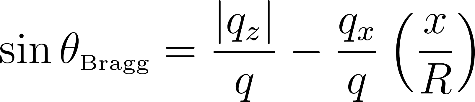
There is an effect which could cause this x-dependent shift, which is the horizontal equivalent of beam dispersion. Horizontally, the phase fronts of the X-rays are circles with radius R. Under conditions of ideal alignment, the effect of this is second order in x/R which is negligible, but if there is a non-zero ꭕ angle then a first-order term appears proportional to x/R and ꭕ. Since ꭕ changes sign under a 180o flip, this can produce the effect seen in the above difference plot. Taking into account the horizontal dispersion in the incident X-ray beam direction, Eq. 2 becomes
(19)
where the effect of the vertical dispersion of the beam (term proportional to y) has already been taken into account as part of the dispersion correction. Using Eqs. 3-4 to evaluate qx leads to
(20)
where I dropped terms that are second order in small angles. Therefore, in addition to the y-dependent shift in the θ of the diffraction maximum away from the ideal theoretical value θBragg, there is also an x-dependent shift proportional to sin ꭕ / R. Since that term changes sign under a 180o flip, the 3 urad/mm in the difference plot, the value of sin ꭕ / R for JD70-101 is 1.5 urad/mm, giving ꭕ = 2.2o which is eminently plausible.
Where should this correction be applied? I hesitate to put it into rcfitter and incorporate it into the primary topographs as I did with the vertical dispersion because, unlike vertical dispersion which is an intrinsic feature of the beam, the horizontal divergence correction depends on the alignment of the target crystal during the scans, becoming zero under ideal alignment conditions. So far, the following variations on the basic hmu histograms are saved in the results files:
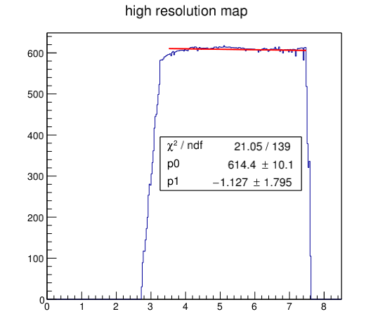
Round 5 only exists because the rcpicker software did not include the dispersion correction when round 3 topographs were produced. In the future, round 3 will include the dispersion correction and round 5 will be eliminated. I debated adding a new round to incorporate the horizontal divergence correction but decided against it because the size of the correction is dependent on details of the analysis which will probably evolve over time. Instead, I will incorporate the correction as a part of Couples::getmap, whenever it is asked for a map with a name starting with hmu. Below I show the corrected difference topograph and x-slice with linear fit after the horizontal divergence correction has been applied. The fix is good.
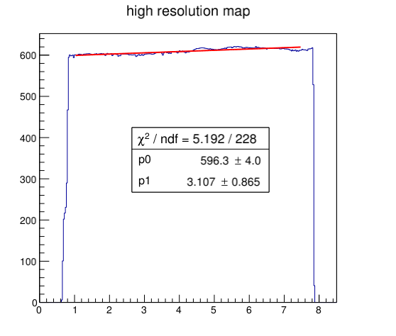
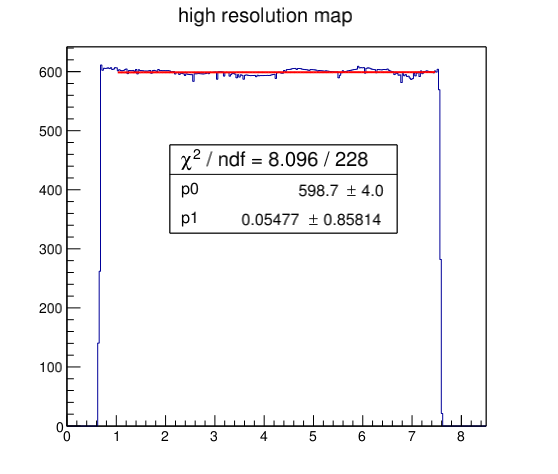
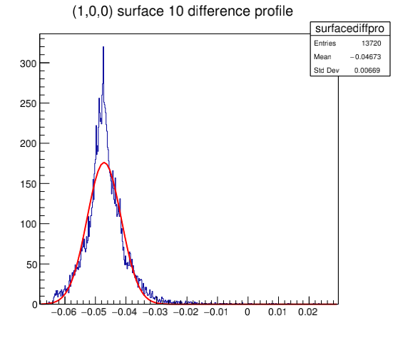
After all of these corrections, we finally have an independent estimate of the systematic error on our rocking curve θ formed from a 1D projection of the difference topograph on the left.
If all instrumental errors were negligible and the crystal were perfect, this distribution would be flat-topped having a full-width of 3.6 urad corresponding to the Darwin width of ideal diamond (2,2,0) at 20 keV. Most of the broadening seems to come from the region close to the glue joint, where the diamond is most distorted, so I look again at the profile excluding the diagonal band 1mm wide along the lower right corner. This did not change the width significantly, going down from 7.0 to 6.7 urad. Most of the instrumental broadening seems to be coming from the motor nonlinearity whose effects are visible as the texture in the 2d color plot of the difference topograph. That being the error on the difference of two scans, the systematic error on each one is that value divided by the square root of 2, or 5 urad.
A detailed error analysis of this sort was never done on the data we took at CHESS, but the systematic error there was probably somewhat better, owing to the high-precision 4-circle goniometer we had on that beamline. I believe that this is as good resolution as can be had with this setup that we have on the BMIT beamline at CLS. It is certainly good enough for the purposes of GlueX. I move on to analyze the remaining scans.
I had originally intended to be able to independently measure the d-spacing and the geometric deformation of the crystal planes using these sets of 4 complementary scans that we collected during the cls-6-2019 run. Unfortunately, it seems that the particular choice of orientations that we used precludes the empirical separation of d-spacing from bending strain. There is a total of 8 possible orientations for the diamond targets, from which we chose 4 during the run. It turns out that the way we took them, in pairs that are flipped by 180o relative to one another around a horizontal axis, are completely redundant with respect to the information that they carry about the crystal. On the other hand, we could have taken them in pairs flipped relative to one another by 180o around a vertical axis, in which case the bending strain would have changed sign whereas the d-spacing strain would not. This is not what we did. However the data we do have are redundant in this way, and so we have independent verification of the systematic errors for each scan, which we can then reduce by averaging. This also brings the advantage that we can extract the vertical dispersion and the horizontal divergence of the beam independent of any assumptions about the quality of the diamond target.
There are other means for testing whether a region is shifted in θ because of bending strain alone, or whether d-spacing changes are also in play. Although these are model-dependent, they will be useful when it comes to analyzing the results from the later scans in cls-6-2019, particularly JD70-100 and JD70-104.
July 12, 2019 [rtj]
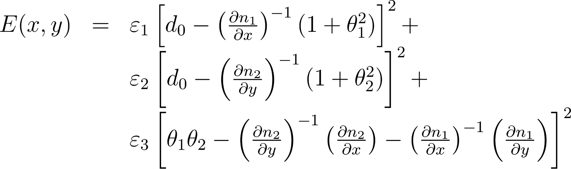
To investigate the role played by crystal defects in the observed rocking curves for a thin diamond, I propose the following general two-dimensional model for the geometry.
(21)
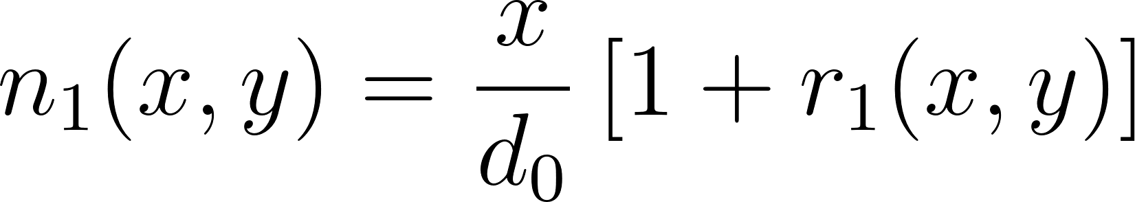
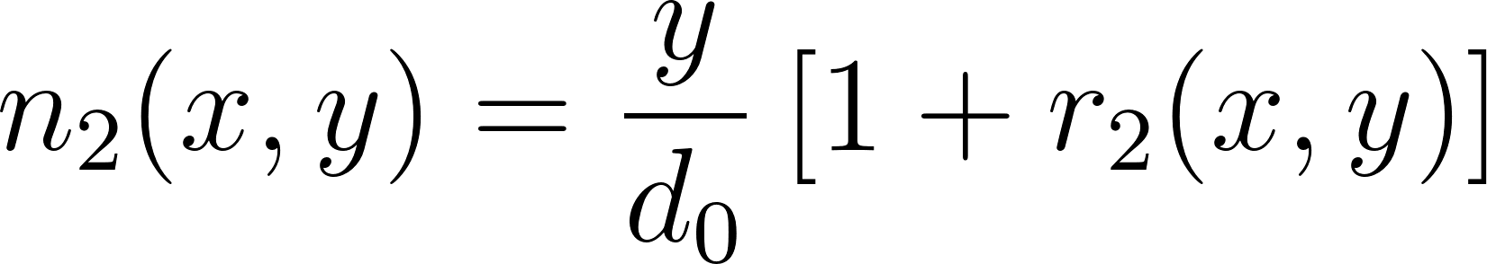
Terms proportional to ε1 and ε2 measure the in-plane deformation energy of the unit cell expansion/contraction along the x and y directions, and the term proportional to ε3 measures the energy of deformation arising from the skew of the unit cell from right-angle corners. The two fields n1(x,y) and n2(x,y) are real number fields that coincide at the corners of the unit cells along the x and y directions with the unit cell indices. The fields θ1 and θ2 are the angular tilt of the u1 and u2 directions above the mean x,y plane of the crystal. Eq. 21 contains only the energy that comes from in-plane distortions of the crystal from its ideal geometry. Additional terms that add stiffness to the plane will be considered later, as a supplement to the thin-crystal model.
Eq. 21 is the free energy density whose integral over dx dy should be minimized to find the stable geometry subject to appropriate boundary conditions. For the present purposes, I consider a finite sheet with small deformations away from the stable equilibrium. Let
(22)
defined such that the new set of variables r1, r2, θ1, θ2 all zero define equilibrium for the system in the absence of defects. To leading order in the perturbations, the Euler-Lagrange equations for this energy density are as follows.
(23)
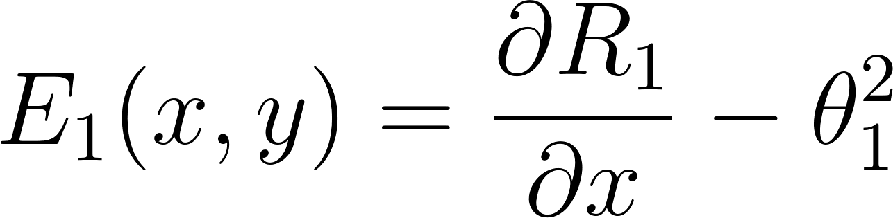
In terms of Euler-Lagrange dynamics, the last two equations in Eq. 23 play the role of constraints, as spatial derivatives of θ1 and θ2 do not appear in E(x,y). The following three basic combinations of fields appearing in Eq. 23 constitute energy density coming from the in-plane strain of the crystal.
(24)
where R1=xr1 and R2=xr2. If all three Ei were zero everywhere, that would automatically solve all four of the Euler-Lagrange equations in Eq. 23. But since there are 4 fields and only 3 equations, the solution is not unique. There is actually a fourth source of strain that enters for crystals of finite thickness that comes from bending.
(24b)
Including a term proportional to E4 in Eq. 21 is needed to make the stable shape unique.
(25)
Eq. 25 leads to the following replacements for lines 3,4 of Eq. 23.
(26)
July 13, 2019 [rtj]
The goal here is to see if we can use the rocking curve measurements of θ1 and θ2 to yield any knowledge of the unknown functions R1 and R2 that contain information directly about the in-plane strains within the crystal that are the source of the distortions from planar geometry. In terms of a perturbation series, if the functions θ1 and θ2 are of order ϵ then R1 and R2 enter at order ϵ2 according to Eq. 23. Our measured deviations of θ1 and θ2 from the mean plane are of order 1 mrad, so according to this model, the dimensionless parameters r1 and r2 that represent the fractional deviation of the unit cell dimensions from the mean are of order 10-6. On the other hand, Eq. 1 shows that in Bragg diffraction the effects of θ1, θ2 (which add to θBragg ) and r1, r2 (which rescale q with factor 1+r) are to shift the rocking curve peak, all four of them at first order. But according to the thin-crystal model, perturbations in θ1, θ2 that are produced by crystal distortions are a factor 1/ϵ (three orders of magnitude) larger than the perturbations that occur in r1, r2. This means that the effects of crystal imperfections on rocking curve peak data is essentially all a by-product of the non-planar plastic distortions that they induce in the shape of the thin crystal.
Hence the only access to r1 and r2 (or equivalently to R1 and R2) that we have using these data is to treat them as the source for the observed θ1 and θ2, and use a thin-crystal model like the one described above for their estimation. If this model holds, our failure to make a complete set of complementary scans to enable the empirical separation of r-dependent and θ-dependent peak shifts does not make any difference in practice; the r-dependent shifts are normally too small to resolve apart from the θ-dependent shifts they induce. The one possible exception to this might be the 20 micron sample JD70-104 that showed the most severe effects from radiation damage. Even in that case, it is doubtful that we would be able to resolve the small shifts coming from d-spacing changes, given that one is measuring the centroid of a broad peak in the region of high radiation damage.
Can we reliably extract information about the crystal defect structure from these rocking curve measurements?
This is the principal question that remains to be answered. The first step is to see if there are any predictions that this 2D model makes that can be checked with our data. In Eq. 26, the left-hand sides of both expressions are first-order in the perturbation, whereas the right-hand sides are third order. For a perturbation expansion to make sense, we should see that terms in θ1 that are proportional to xn or in θ2 that are proportional to yn with n>1 should be small. The figures below show several slices of θ1 at fixed y (left) and θ2 at fixed x (right) taken from scans 40 and 10 of JD70-101, respectively. Violations of the model constraint appear as deviations from linear behavior in these curves. While there are a few of these curves that appear linear, there are deviations from linearity that go well beyond what I would expect based on thin-crystal perturbation theory.
Based on this observation, I will not pursue any further the idea that I can extract detailed crystal defect structure information from the shapes of these θ1 and θ2 topographs. This simple 2D model analysis shows that the geometric deformations we observe are not explained merely as a consequence of in-plane stresses being relieved through out-of-plane plastic deformation in a thin crystal. Out-of-plane stress forces must also be in play, to produce the complicated shapes we see. These θ1 and θ2 topographs do not contain enough information to constrain a full 3d model of these crystals, so at this point I give up any further investigation along these lines.
July 11, 2019 [rtj]
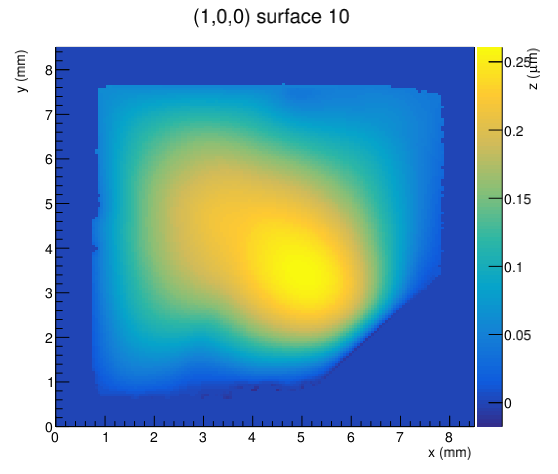
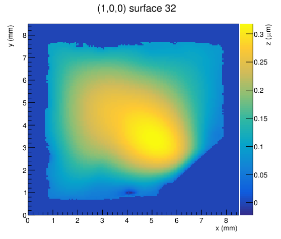
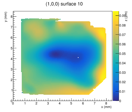
Since the two pairs of x,y scans are fully redundant the way we took them in the cls-6-2019 run, this gives us an independent means to determine our final measurement errors on the extracted shape of the (1,0,0) planes that comes out from the geometric model analysis described above, where all of the local variation in the rocking curve peak position is attributed to bending strain that is smoothly distributed over the surface of the diamond. Here are the results from a reconstruction performed with a resolution of 150 x 150 pixels covering a field of 8.5 x 8.5 mm2 for sample JD70-101.
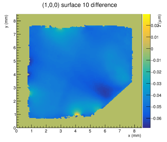
The boundaries of the diamonds in the two figures are derived independently, using the topograph images from each pair of scans. Because the beam was not always perfectly centered on the diamond, there were sometimes regions of the diamond that saw very little beam intensity, and where the fits were sometimes unable to pick out the peak. In spite of that, it is clear from a visual comparison of the above plots that the two profiles are of the same diamond in the same orientation. Differences in the color maps that are apparent in the side-by-side comparison above are mostly due to the different (and arbitrary) tilt and vertical offset of the two solutions. The difference left - right is shown below, after calling Couples::level take out most of the difference that comes from independent tilts.
The mean value in the difference plot profile (right plot) is arbitrary, but the standard deviation shows the measurement error on the computed surface, which is 7 nm. This is really very good, better than I had dared hope to see! The maximum deviation from a plane obtained for this JD70-101 sample is about +/- 125 nm, with a resolution of 7 nm.
I then proceeded to apply the above analysis to the remaining 4 virgin samples that were scanned during the cls-6-2019 run. All of these results are saved in a new set of root files, one per sample, saved under the name JD70-XXX_couples.root in the cls-6-2019/results directory on dcache. This is the same folder where the JD70-XXX_yyy_rocking_curves.root files are saved, and the JD70-XXX_yyy_results.root files. Figures similar to the ones shown above for JD70-101 are also saved together with the original rocking curve topographs in the web directory /halld/diamonds/cls-6-2019, which is linked from the inventory spreadsheet.
July 17, 2019 [rtj]
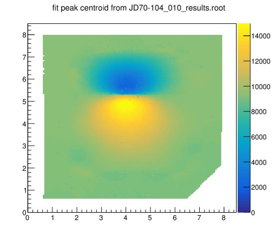
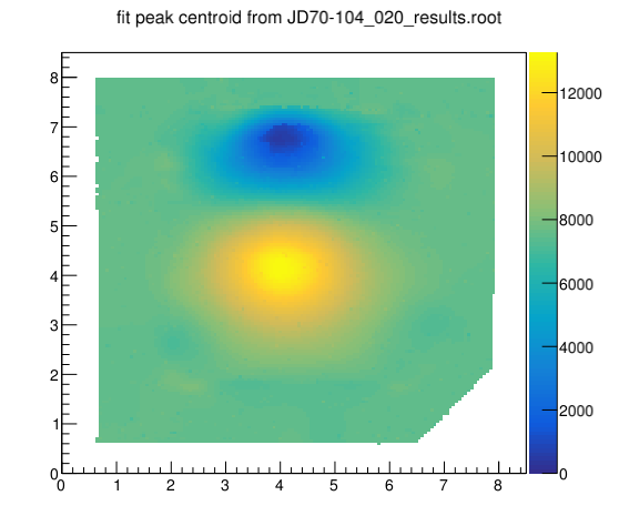
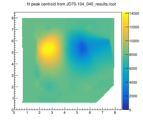
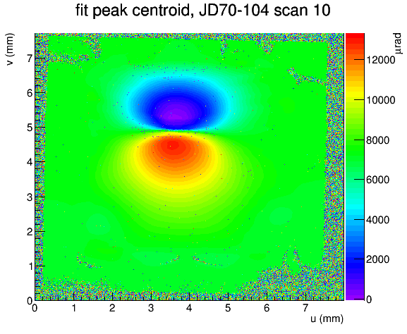
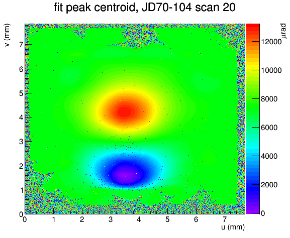
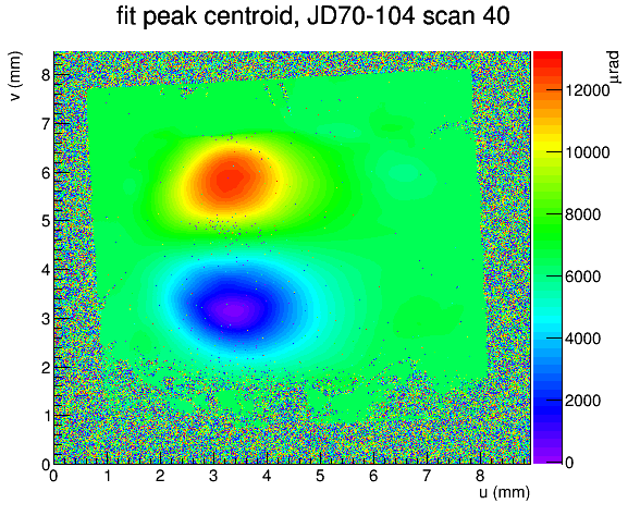
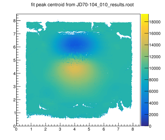
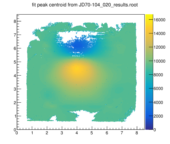
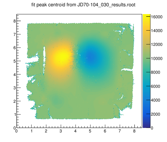
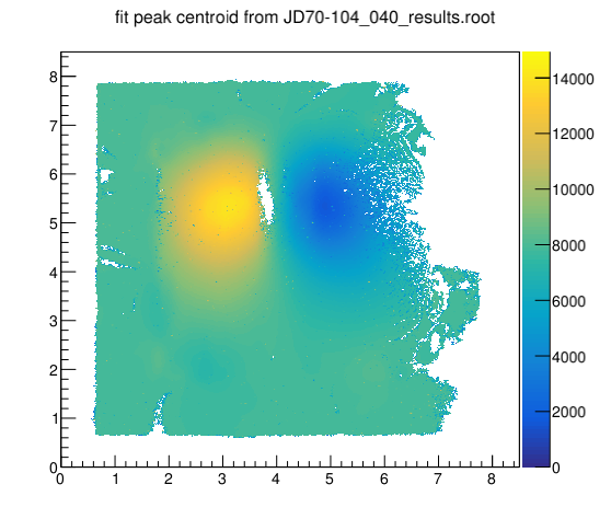
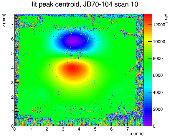
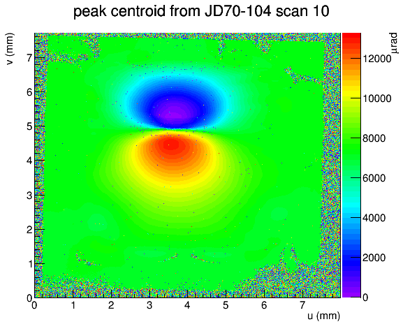
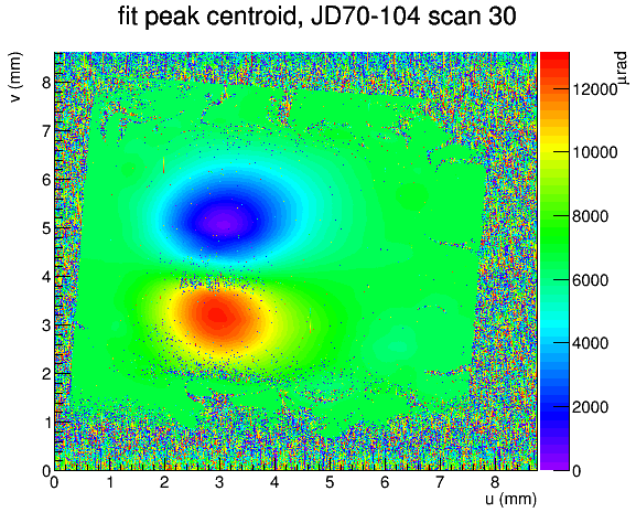
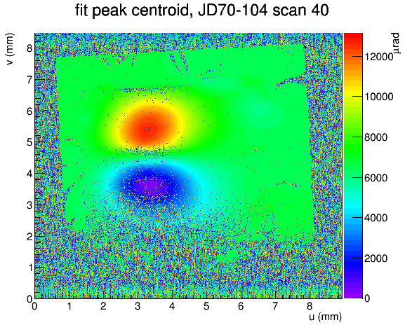
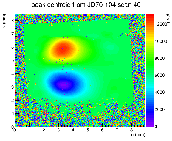
Today I realized that there might be another method for extracting shifts in the d-spacing from the measurements we took during the cls-6-2019 run. I came across this effect by accident, when I noticed a big discrepancy between complementary scans we took of JD70-104. The images below are the peak mean topographs for JD70-104 from the cls-6-2019 run. These topographs have many voids in them, where the fitter was unable to find a peak, so I filled them in using the Map2D::FillVoids() method to make the effect more visible.
Scans 10 and 20 are both reflections from the same lattice vector, with the sample flipped around the horizontal axis perpendicular to the beam. The right image has been inverted in the vertical direction to make it directly comparable to the left image. The only difference between the two scans is which side of the diamond is facing upstream in the X-ray beam. Notice in the left image how there is a near-discontinuity around y=5.3mm, whereas in the right image the two extrema are well-separated.
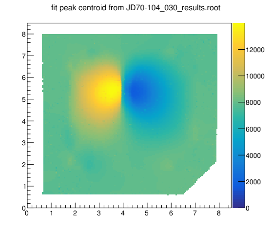
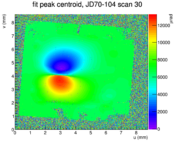
The effect is even more pronounced for scans 30 and 40, shown below. Here the fitter has produced what looks like a discontinuity where the high and low angle regions meet around x=3.8mm. This is not a real discontinuity; see the raw images below to see what the hmu topographs look like before running FillVoids(). In spite of the steep rate of change of peak θ in this region, sweeping the mouse in rcpicker through the region between the yellow and blue blobs reveals a smooth transition.
The comet-tail in the right plot below is an artifact of the FillVoids algorithm trying to guess what belongs in this region where no diffraction peaks were found; the right-most 20% of the pixels in scan 40 are mostly just noise in the raw data.
The correction that must be applied to remove this image distortion is as follows.
(27)
where L is the distance from the sample to the scintillator plane of the camera, and θBragg is the Bragg diffraction angle corresponding to the selected reflection. Notice that θBragg is not the measured θ angle of the target stage, but the true Bragg angle of the diffraction process. The θ angle of the target stage has the non-planar distortions of the diamond (2,2,0) planes in it, whereas the Bragg angle is only a function of the d-spacing of the crystal and the X-ray energy, as specified in Eq. 1.
This means that d-spacing variations across the surface of the diamond would generate spatial distortions in the diamond image that push patches with similar d-spacing up or down in the topograph, relative to the outer frame regions where the d-spacing should be uniform and ideal. This highlights a key difference between the effects of plastic deformation of the crystal planes and d-spacing variations that I did not recognize earlier when I first considered how to extract d-spacing variations from rocking curve data. Plastic warping of a thin diamond generates spatial variations in the motor stage θ of the local diffraction maximum, but it does not affect the 2θ deflection angle of the X-rays, whereas d-spacing variations do. Might local d-spacing shifts in the region of the irradiated beam spot in JD70-104 explains the differences between the left and right plots shown above?
July 18, 2019 [rtj]
A second prediction of the d-spacing variation hypothesis for the origin of the differences between the complementary topographs of JD70-104 would be that there should be regions in the topographs where the pixels see no diffracted intensity (voids) and other regions where individual pixels see more than one peak where the displaced patches overlap. To look for this, I go back to the raw topographs of mu, the mean θ of the primary peak found for each pixel.
These are raw images so the sample orientations are different in each image, but the left-right pairs of images correspond to complementary scans, where the diamond was flipped over around a horizontal axis and the same reflection was scanned through a similar angular range. The contrast in terms of the separation between the two blobs is clearly visible in these raw images. There are voids visible in these raw images, but they appear mostly in the regions of the frame around the outer edges. These voids cannot be the result of image deformation arising from d-spacing variations because the frame consists mostly of virgin diamond.
Using the rcpicker tool, I was able to ascertain that the interior voids that appear in all of these images are the result of the coarse step size that was used for these scans, which was a factor 4 larger than what was used for all of the other scans, otherwise they would have taken hours to complete. The peak width is less than 10 urad for most pixels around the frame region, which means that with a step size of 9.76 urad, we might step right over the maximum, particularly if the maximum appears in the part of the stepping motor nonlinearity cycle where the steps are larger than average. Because regions with narrow rocking curves do not exhibit rapid spatial variations, using FillVoids to extrapolate from neighboring pixels to fill in these void regions is appropriate.
What is not so clear is what is going on in the region between the two bright blobs, or how Eq. 27 explains the appearance of this strong dipole pattern. If radiation damage is breaking the bonds of the diamond crystal, which is what one might expect based on the fact that diamond is over-dense at standard pressure, one expects that the d-spacing should exhibit a local increase in proportion to the radiation damage sustained. This would produce at least 2 effects:
Such a bubble or dent would produce the dipole dip/rise pattern that we see in these topographs. The fact that the overall pattern is the same in x and y is further support for this geometric interpretation. But what would cause the blobs to shift in opposite directions when the target is flipped front-to-back by 180o around the horizontal axis? Effect #1 should produce a uniform shift toward the red in both lobes of the dipole pattern, and shift/compress the pattern toward larger y in the center of the spot. This would have the visual effect of stretching the red blob vertically, and making it appear larger and deeper than the blue blob, assuming a symmetric bubble. The direction of the effect would be reversed in the flipped geometry, which would make the center of the dipole pattern appear to shift between the two images, once the right one has been inverted to permit a direct comparison. The presence of all of these void regions in the two topographs partially obscures the comparison, but both the x and y scan pairs show the same unmistakable effect, that the separation between the two blobs is very different in the two orientations, while the midpoint between their centers is the same.
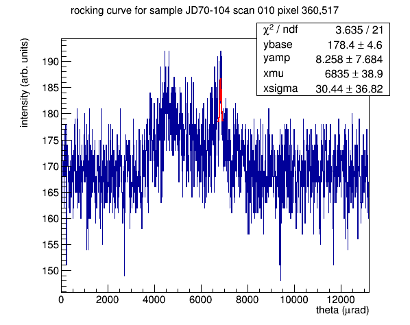
This would seem to rule out d-spacing variations as a simple explanation for this difference. If there were appreciable d-spacing variations arising from Eq. 27, one would expect somewhere in the images to find pixels whose rocking curves have two separate peaks, coming from different regions of the crystal diffracting at different Bragg angles so that they both illuminate the same spot on the camera scintillator. Searching for pixels with double peaks with rcpicker, I found the following examples of this in the region between the blobs in hmu topographs from scans 10 (upper plot below) and 30 (lower plot below).
These peaks are extremely broad, normally associated with a large curvature of the crystal in this region. Examples like the ones shown above are not difficult to find by scanning the pixels in the cross-over region from the blue to the red blobs in scans 10 and 30, most of the pixels in this region do not show double-hump patterns like these, but consist of a single broad maximum like one of the two peaks shown in these plots. Given that double-peak curves like these are the exception rather than the rule, I will not attempt to build a general explanation for the observed pattern based on them.
Thinking more about this effect, there is no simple geometric explanation for it because the way I am viewing the effect it violates time-reversal symmetry. If passing X-rays through the same region of a sample in forward and reverse directions gives a different result, as these complementary topographs suggest, then time reversal symmetry is violated. There must be a more banal explanation.
These images are actually the sum of a large number of monochrome images, each of a different color. At the extreme blue and red ends of the spectrum, only a single dot at the center of one of the two blobs is present in the monochrome image. Because these two extreme colors are so far from the average color (green), what if the position of the diamond edges in the red and blue slices do not align with each other at the camera? This would happen if the target is displaced from the center of rotation of the theta rocking stage. I remember checking this during setup for the June 2019 run, and concluding that the target is within 5 cm of the center of rotation for the theta stage. If I suppose that it is 5 cm above the center of rotation then a 10 mrad rotation in theta might produce a shift of 120 microns of the image outline on the camera surface. This is the right order of magnitude!
The following figure is useful as a guide for how to correct for this effect.
(28)
Now operating under the assumption that θBragg is a fixed constant for all of these samples, I obtain a slope for the walk of the topograph image in y as a function of θ.
(29)
where θ0 is the mean value of θ for a given rocking curve scan, and Δθ is the difference θ-θ0 for any given step in a scan. The exact value of this vertical image walk is different for every scan, but a typical value might be 15 um/mrad. For typical scans spanning a total of 1-2 mrad, I can see how this systematic might not have been noticed, whereas it stands out like a sore thumb when the scan length reaches 20 mrad in the case of JD70-104. Having uncovered it, I will now incorporate a correction for it into the analysis of all of our samples.
The sign of the y-walk coefficient is not determined by Eq. 29 because it is not known whether the center of rotation of the θ-stage is above or below the beam center. It is also not known whether the sample is in the plane containing the theta axis, as shown in the figure, or behind the plane or in front of it. Any displacement of the target from the plane containing the pivot is another source of the same kind of walk. All of these effects can be carried by designating the coefficient of Δθ in Eq. 29 to be a constant across and entire scan, and determining its value empirically for each scan. In the case of the JD70-104 scans, I will assume that the same value applies to all 4 scans, and then assume the same value for all of the other targets that were studied in the cls-6-2019 run, since a uniform target geometry was used for all scans during that run period.
July 19, 2019 [rtj]
I modified the Couples class to incorporate a correction for the vertical walk of the target image with θ and experimented with a range of values for the gain constant dy/dθ. The plots below were obtained using dy/dθ = -0.075 mm/mrad.
The blob alignment now looks much better between the two left-right pairs. But there are now artifacts of the transformation visible in these images, notably the vertical streaks between the two blobs in the scan 10 topograph, and horizontal streaks in the scan 30 image. These come about because of the extreme stretching of the pixels in that region.
This is a good way to estimate the size of the effect, but a much better way to make this correction would be to go back to the original rocking curve data and make the correction there before the fits are carried out. The extremely broad enhancements seen in the 1D projections on p. 38 and 39 are actually the superposition of the enhancements across an entire region of the sample, piled up into one pixel by the walk of the image nearly canceling the movement of the enhancement across the image.
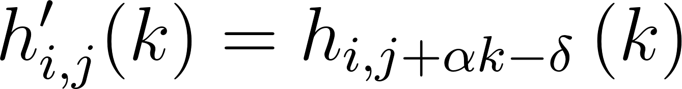
I now go back to the original raw image data in JD70-104_XXX_rocking_curves.root and add a second instance of the rctree in which the 1D histograms from the individual camera pixels are cut and spliced in y-columns, as follows.
(30)
where the walk constant ꭤ=0.0813 pixels/step corresponding to -0.075 mm/mrad assuming a pixel size of 9 microns and a step size of 9.76 urad for these scans. This transformation chunks up the raw 1D histograms into sections of roughly 12 steps each, and shifts each successive section to the next pixel down. This will shift the entire image down by 0.5 mm in y, which I compensate by splitting the difference with δ=56 so that the average position of the sample within the camera frame is unchanged by the transformation of Eq. 30.
The transformation in Eq. 30 was implemented in a new class rcshifter.C which reads from JD70-104_XXX_rocking_curves.root and writes its output back out to a new instance of rctree within the same file. It needs to work from a local copy of JD70-104_XXX_rocking_curves.root for this to work. In this way, the original and the shifted versions of the raw data are both saved side-by-side in the rocking curves root file in case at some point one would like access to the original unshifted data.
July 20, 2019 [rtj]
Testing my new rcshifter on the JD70-104 scans, I discovered that this procedure comes with problems of its own. Certain pixels in the camera are very noisy, and have a much higher noise baseline than their neighbors. Before the shifting operation, these pixels only generated a single noise point in the topograph, which was easily removed by clipping spikes in the output image. Now those noisy channels have distributed their noise over a vertical stripe of 112 pixels in height, which is much more troublesome to remove and very distracting to the visual quality of the image.
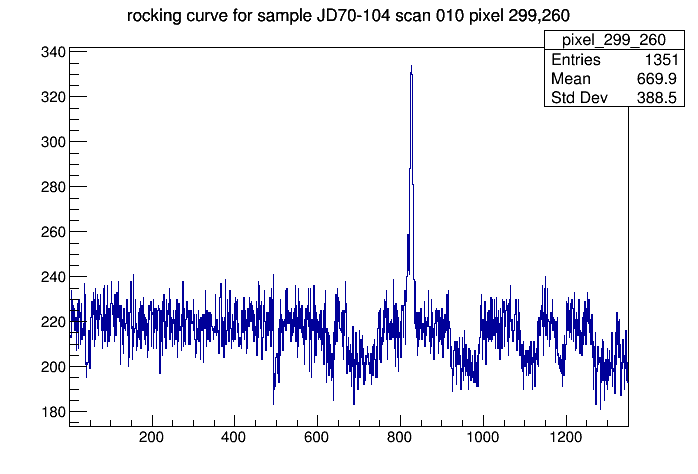
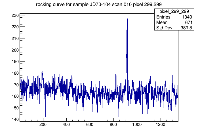
Below I show the impact of noisy pixel 299,261 seen in JD70-104 scan 10. Normal pixels show a noise floor around intensity 165 adc units, whereas pixel 266,261 has a noise floor up around 220. This does not give the appearance of a false peak before the y-walk correction because variation in the noise floor within a single pixel is generates structures that are too broad to mistake for a diffraction peak. After the y-walk correction (second plot below), the noisy pixel at 299,261 now appears as a narrow spike in the channels above and below it, as e.g. is seen in the rocking curve for pixel 299,299 post-correction as a narrow spike around channel 195.
This spike around step 195 in the 299,299 rocking curve would probably not be fitted because of the much larger (true) peak around step 900, but it is the second largest peak in the distribution.
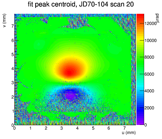
In general, the noise baselines are much more rough after the walk correction than they were before, which probably means that the peak finder will be less reliable in finding and fitting the diffraction maximum. So even though it seemed that shifting the raw data is a more correct way to remove the y-walk, in practice I may get better results by fitting the uncorrected data and then removing the walk from the hmu topographs as I did with the earlier approach. Below I show the results of the fit to y-walk corrected raw rocking curves (left) with the original fits to the uncorrected rocking curves (right). Both plots show the theta of the diffraction maximum encoded in color according to the color map displayed to the right of the plot.
As expected, the defects in the right plot are exaggerated in the left plot. Below I show a similar comparison between corrected (left) and uncorrected (right) fits for the complementary scan 20.
The blue blob in scan 20 is badly messed up by the correction, in contrast to the uncorrected image at the right. This is also true in when using the original treatment of the correction, as seen in the image for scan 20 shown on p. 41. The remaining two scans are shown below.
I am keeping both sets of results because each might have advantages in one or another context. The results with the y-walk correction applied prior to the fit (left column of plots above) I save under the sample name JD70-104-ywalk, keeping the prefix JD70-104 for the fits performed on the uncorrected images. It might be possible to go back to the peak finding and fitting algorithm and improve its performance on these noisy y-walk corrected data, but I have already spent considerable effort to optimize it in the past, and doing better might require a lot of effort where it is not really needed.
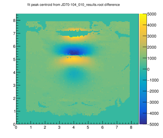
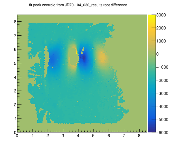
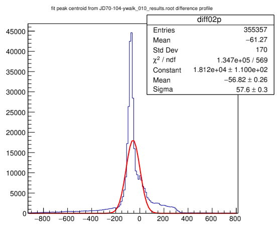
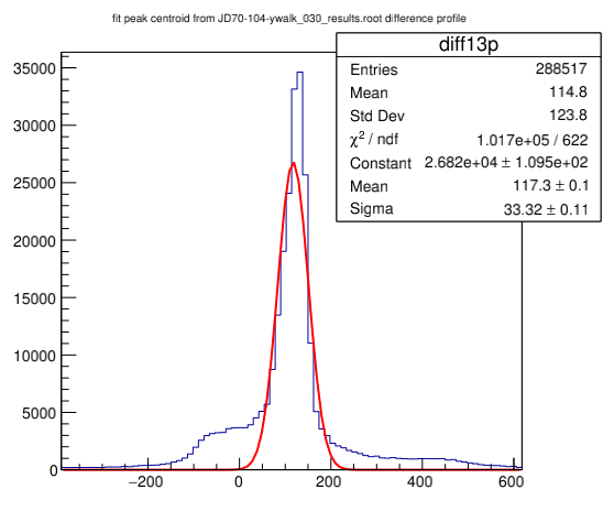
The one remaining question I would like to answer using these y-walk corrected fits is what level of consistency we obtain between the complementary scans. In the case of the virgin diamond scans, the RMS difference between the two complementary scans was in the range 4-8 urad, with scans of step size 2.2 urad. The JD70-104 scans were taken with 4x the step size, and I was unable to correct for the motor nonlinearity with such a coase step size. Based on this, I might hope to find a consistency a factor 10 worse, so something at the level of 40-80 urad. The difference results obtained with the y-walk corrected fits are shown below.
These are what I see after doing the best I can to line up the images of the diamonds in the two complementary pairs, and then subtracting the two topographs 0-2 and 1-3. While these RMS values around 40 urad are at the low end of what I predicted, they should be taken as only a rough indication of the true uncertainty for two reasons,
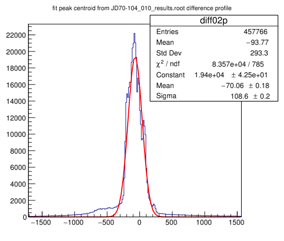
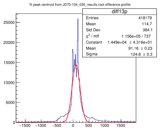
In contrast with this, I have made the same difference plots for the results where the y-walk correction was applied to the topograph images, after the fits were performed on the uncorrected rocking curves. Here the pixel coverage is higher, but the analysis is subject to additional systematic errors.
While the RMS widths of the main peaks are a factor 2-3 larger for the post-fit analysis than was seen in the pre-fit correction results, the total number of pixels compared is also substantially higher in the post-fit analysis results, as reflected in the total number of entries (top line in the statistics box for each plot).
July 22, 2019 [rtj]
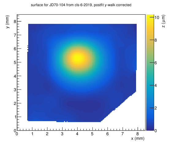
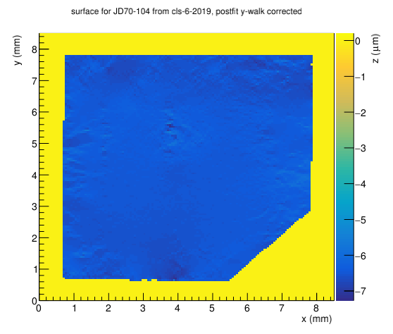
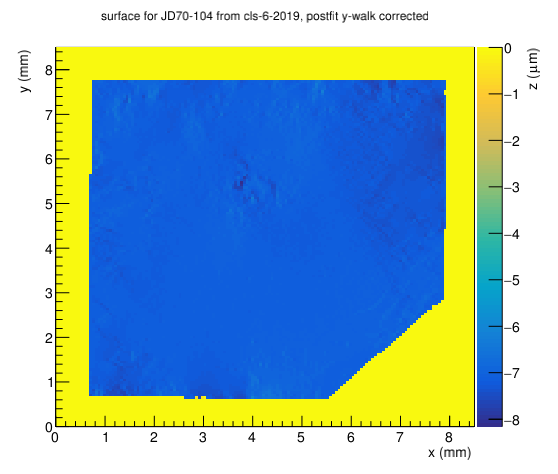
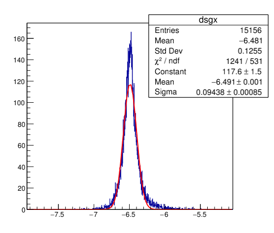
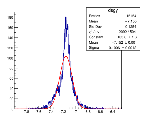
JD70-104 is the best sample we have for validating the software that solves the differential equations for the shape of the crystal geometry that gives rise to the measured rocking curve topographs. To make up for the significant voids in these topographs, I want to combine the complementary scans into one each for x and y, then apply Map2D::PoissonSolve to the two combined maps. I try this first for the post-fit correction results because the coverage is more complete for those topographs. Here is the result for the solution surface, followed by the difference maps between the input hmu topographs and the gradients of the solution. The consistency is right around 100 urad, which is the estimated error on the input topographs. This consistency is a strong confirmation that the geometric model we are using here is sufficient to explain all of our rocking curve measurements, even when severe radiation zones are present.
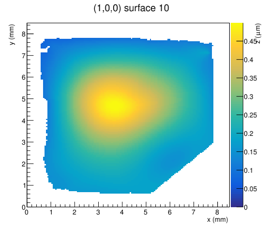
The solution reveals a rising of the (0,0,1) plane near the center of the beam spot by about 10 microns above the average height of the central membrane around the edges. This is large enough that it should be clearly visible using the Zygo. Seeing this geometric deformation in the Zygo would be a good cross-check on the validity of this analysis.
The appearance of a hump (or dimple) appearing as an out-of-plane plastic deformation of the crystal planes at the location of the beam spot that is seen in JD70-104 seems to be a generic result seen in any sample that has been exposed to the beam. Below I show surface shapes for JD70-100 (first plot) and JD70-105 (second plot). These are thicker targets (50-60 microns) but they have also seen a substantial amount of time in the Hall D beam. JD70-105 looks like there is more than one beam spot, suggesting that the spot was moved at least once over the time period that this radiator was in use. The direction of deflection for the two samples (up vs down) are opposite, and is expected to be random, depending on the details of the longitudinal strain profile in the crystal.
The height of the deformation in JD70-100 is a factor 5 higher than JD70-105, as expected from the fact that all of the radiation dose in JD70-100 was deposited in the same spot, and JD70-100 saw more beam than JD70-105 did. It would be interesting to compare the total charge seen by these two samples as a means for estimating the rate at which the deformation with increased radiation dose, and whether there might be a threshold below which no effect is seen. This is question A4 listed in the analysis goals section of this logbook. Before I look at that, I want to address question A3, which concerns a comparison with the results for samples JD70-101, 103, 106, 107, and 109 that were taken during run cls-11-2017.
Based on a preliminary look at the raw topographs that we took of the 5 virgin samples at CLS in November, 2017, I concluded that we had done a terrible job epoxying the samples to their aluminum tabs, and that they would not be usable as radiators for GlueX until they had been remounted and rescanned. Was that conclusion justified? Did the more careful job we did when we remounted these samples prior to the June, 2019 run make a noticeable difference in the observed plastic deformation? Was the net effect of the epoxy removal + cleaning process + remounting procedure an improvement in the plastic deformation, or was what we saw in 2017 the result of intrinsic strain within the samples that was largely unrelated to the size and spread of the epoxy spot?
To answer these questions, I go back to the cls-11-2017 results and create new Couples objects for these scans. These were all taken in complementary pairs, as was done in June 2019, so the same software tools should work there without modification. The contents of the results.root files are different for this run because I was not doing the run_normalize step in run_rcfitter.C at the time I ran the fits. I went back and ran run_normalize against all of the topographs in the results.root files from cls-11-2017 to put them on the same footing as the cls-6-2019 results.root files, then ran destripe against them and pushed them back to the results directory on pnfs.
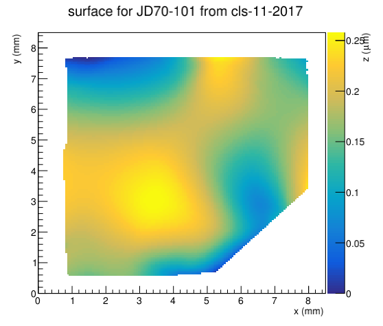
July 27, 2019 [rtj]
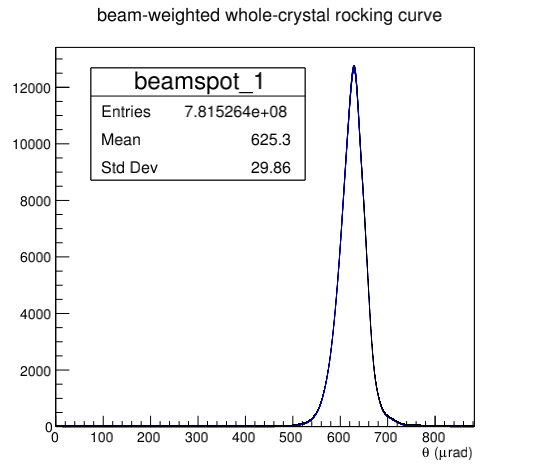
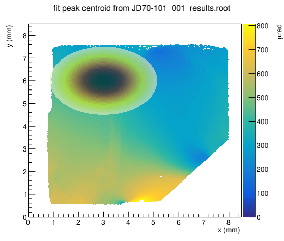
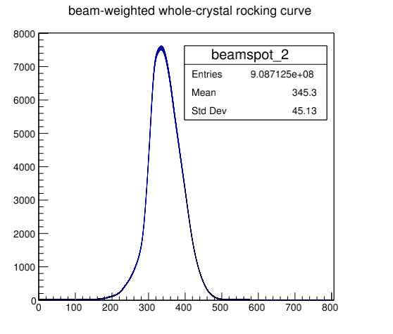
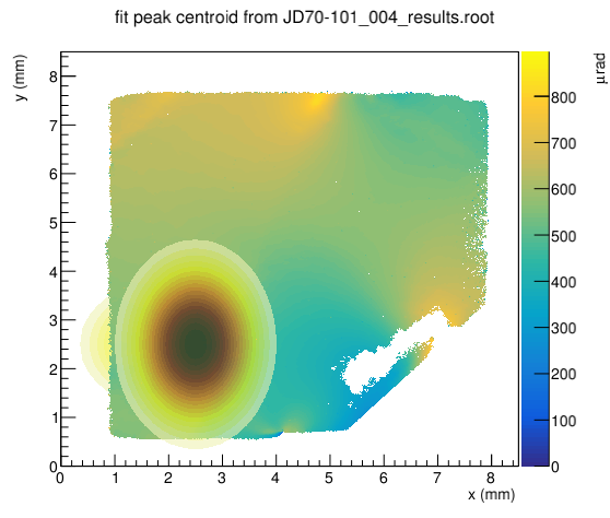
The plot on the right above is of the same sample JD70-101 from run cls-6-2019. Clearly the two surface shapes are different, showing the importance of how the sample is mounted to the final plastic deformation of the surface. The surface at the right has much greater local variation and smaller regions of maximum and minimum height, compared to the one on the right. This difference is further borne out by the following beam-weighted rocking curves evaluated for the samples at the same beam positions.
July 29, 2019 [rtj]
First I show the beam-weighted whole-crystal rocking curve for JD70-101 derived from the scans taken in run cls-11-2017. A variety of different beam positions are shown, each one with both PARA and PERP orientation topographs and summed rocking curves. Only scans 4 and 1 are shown because part of the sample was hidden by the beam slits in scans 2 and 3.
Below is shown the same pair of scans with the beam spot aligned with the left-hand edge where the curvature of the crystal seems to be less pronounced.
Finally, I show in the four plots below what the whole-crystal rocking curves look like with a beam-weighting gaussian located near the upper right edge of the sample.
In all of these views, the total width of the rocking curve peak is significantly larger than the GlueX design goal of 20 urad. The variation in the beam-weighted width across the usable area of the crystal is roughly a factor 50%, from the best-case of 33 urad along one of the projections in the left-hand edge position to the worse-case of 47 urad in the orthogonal projection in the same beam position.
Was there any quantitative improvement seen for the same sample following the remounting operation in June 2019? Here are similar plots for JD70-101 derived from cls-6-2019 data. These data show no improvement in the 2019 data over 2017, but in fact the rocking curves are about a factor 2 worse! This is qualitatively consistent with the fact that the scan lengths recorded for this sample in the cls-11-2017 logbook are a factor 2 shorter than those recorded for the same sample in the cls-6-2019 logbook.
Might there be an error in the two scales? The motor settings were completely different in the two runs. If so, this should be visible in a comparison of the single-pixel rocking curve widths, since it is difficult to see how that would be changed by any remounting procedure. I compared 1D projections of the hsigma_moco topographs for all 4 scans of JD70-101 from cls-11-2017 and cls-6-2019, and both agree that the mean single-pixel rms width lies between 7.5 and 8.0 urad. Based on this, I would say the remounting made the flatness worse for this sample.
July 30, 2019 [rtj]
While sample JD70-101 was a factor 2 worse than the GlueX design goal of 20 urad whole- crystal rocking curve width when we first tested it in 2017, when it was retested in 2019 after remounting, the width had grown by another factor 2 to be a factor 4 above the design goal. It is not clear whether this happened as a result of all of the handling that happened during the remounting process, or whether there is an uncontrolled random factor injected each time a crystal is epoxied to its mount. If the first hypothesis is true then we can expect a similar degradation in the cls-6-2019 results for the remaining 4 virgin samples, relative to what was seen in cls-11-2017, whereas the second hypothesis would suggest that one or two of them might have improved. In particular, JD70-107 is an interesting subject because that one I was able to remove from its mount without immersing it in hydrochloric acid to weaken the old epoxy bond. Other than that exception, the procedures for removal and remounting of all 5 virgin samples was the same.
These procedures are documented in more detail elsewhere, with photos. I list them here just as a reminder of the relatively strong measures that were needed to remount these samples.
October 1, 2019 [rtj]
It was suggested by Beni Zihlmann that a Zygo surface profile image of radiator JD70-104 might be able to see the bulge in the middle of the beam spot. James and I took the following 3 radiators down to the Zygo in IMS lab 0012 where the Zygo microscope is now located.
These steps were taken to set up the Zygo for measurements.
Zip all of the above files into a single zip file and copy them onto a thumb drive. These will be copied later into a folder in a work directory on the linux cluster, and analyzed using our own custom stitching software. Do not rely on the built-in stitching algorithm provided by MetroPro.
All of the images we took during these scans were taken with the aluminum mounting tab in the lower right corner of the image. The following convention was used in naming the zip files.
where XXX is the sample id (100, 104, 105), ZZ is the zoom setting (1x, 2x), and S is the side of the sample that is facing up in this view.
In orientation S=b, we placed a folded piece of lens paper under the aluminum tab to prevent it from rocking back and leaving the diamond elevated at an odd angle with respect to the glass slide on which it rests.